Collection Of Papers |
|
© 2017 Benjamin Burkhard, Joachim Maes.
This is an open access article distributed under the terms of the Creative Commons Attribution License (CC BY 4.0), which permits unrestricted use, distribution, and reproduction in any medium, provided the original author and source are credited.
Citation:
Burkhard B, Maes J (Eds) (2017) Mapping Ecosystem Services. Advanced Books. https://doi.org/10.3897/ab.e12837
|
Foreword
The world's economic prosperity and well-being are underpinned by its natural capital, i.e. its biodiversity, including ecosystems that provide essential goods and services for mankind, from fertile soils and multi-functional forests to productive land and seas, from good quality fresh water and clean air to pollination and climate regulation and protection against natural disasters. This is the reason why, for example, the first priority objective of the 7th Environment Action Programme (7th EAP) of the European Union (EU) is to protect, conserve and enhance the EU natural capital. In order to mainstream biodiversity in our socio-economic system, the 7th EAP highlights the need to integrate economic indicators with environmental and social indicators, including by means of natural capital accounting, to measure the changes in the stock of natural capital at a variety of levels, including both continental and national levels.
The EU Biodiversity Strategy to 2020 called on Member States to map and assess the state of ecosystems and their services in their national territory by 2014, with the assistance of the European Commission. The economic value of such services should also be assessed, and the integration of these values into accounting and reporting systems at EU and national level should be promoted by 2020 (see Target 2, Action 5).
This specific action aims to provide a knowledge base on ecosystems and their services in Europe to underpin the achievement of the six specific biodiversity targets of the strategy as well as including a number of other sectoral policies such as agriculture, maritime affairs and fisheries and cohesion.
Mapping ecosystem services is essential to understand how ecosystems contribute to human wellbeing and to support policies which have an impact on natural resources. In 2013, an EU initiative on Mapping and Assessment of Ecosystems and their Services (MAES) was launched and a dedicated working group was established with Member States, scientific experts and relevant stakeholders. The first delivery was the development of a coherent analytical framework) to be applied by the EU and its Member States in order to ensure consistent approaches. In 2014, a second technical report) was issued which proposes indicators that can be used at European and Member State's level to map and assess ecosystem services. The indicators are proposed for the main ecosystems (agro-, forest, freshwater and marine) and the important issue of how the overarching data flow from the reporting of nature directives can be used to assess the condition of ecosystems is also addressed.
From the start of MAES, some exploratory work was undertaken in parallel to assess how some of the biophysical indicators could be used for natural capital accounting. It was also important to ensure that the data flows available at European level and, in particular, those from reporting obligations from Member States would be used for the mapping and assessment of ecosystems and their condition. More recently, dedicated work on urban ecosystems was initiated with the active contribution of many cities and a fourth technical report) on mapping and assessment of urban ecosystems and their services was published. An overlapping activity on the strengthening of the mapping and assessment of soil condition and function in the long-term delivery of ecosystem services is also being developed.
In the context of The Economics of Ecosystems and Biodiversity (TEEB), a study of available approaches to assess and value ecosystem services in the EU was supported by the European Commission to support EU countries in taking forward Action 5 of the EU Biodiversity Strategy.
In 2015, a Knowledge Innovation Project on an Integrated System for Natural Capital and Ecosystem Services Accounting (KIP INCA) was launched jointly by four Commission services (Eurostat, Environment, the Joint Research Centre and Research and Innovation) and the European Environment Agency. This project aims to design and implement an integrated accounting system for ecosystems and their services in the EU, to serve a range of information needs and inform decision making of different policy sectors, building on existing work in EU countries. Important ecosystems services provided by nature will therefore be explicitly taken into account and demonstrate, in physical and to the greatest extent possible in monetary terms, the benefits of investing in the sustainable management of ecosystems and natural resources.
Finally, the European work undertaken under Target 2, Action 5, is actively contributing to major ongoing initiatives, such as the global, regional and thematic assessments under the Intergovernmental Platform on Biodiversity and Ecosystem Services (IPBES) and the UN guidelines on experimental ecosystem accounting from the System of Environmental-Economic Accounts (UN SEEA EEA).
At present, with the constructive support of research and innovation projects and actions, such as ESMERALDA and with the amount of work already accomplished in the Member States and at EU level, the momentum for the next steps is impressive (http://biodiversity.europa.eu/maes/maes_countries).
The policy developments in Europe, but also in many other countries and at global scale, have spurred the scientific community to map ecosystem services, to develop new methods, to assess uncertainty of maps and to provide practical applications of using maps in various decision-making processes. This book is an excellent summary of the achievements of ecosystem service mapping and provides guidance for scientists, students, practitioners and decision makers who need to map ecosystem services.
There are still big challenges ahead of us such as the improvement of the mapping and assessment of the ecosystem condition and the integration of the assessment of the ecosystem condition with ecosystem services and the construction of the first ecosystem accounts. As highlighted in this book, we are however on a very positive track!
Anne Teller
European Commission,
Directorate-General Environment
Chapter 1. Introduction
Ecosystem services (ES) are the contributions of ecosystem structure and function (in combination with other inputs) to human well-being. This implies that mankind is strongly dependent on well-functioning ecosystems and natural capital that are the basis for a constant flow of ES from nature to society. Therefore, ES have the potential to become a major tool for policy and decision making on global, national, regional and local scales. Possible applications are numerous: from sustainable management of natural resources, land use optimisation, environmental protection, nature conservation and restoration, landscape planning, nature-based solutions, climate protection, disaster risk reduction to environmental education and research.
ES maps constitute a very important tool to bring ES into practical application. Maps can efficiently communicate complex spatial information and people generally prefer to look at maps and to explore their content and practical applicability. Thus, ES maps are very useful for raising awareness about areas of ecosystem goods and services supply and demand, environmental education about human dependence on functioning nature and to provide information about interregional ecosystem goods and services flows. Furthermore, maps are mandatory instruments for landscape planning, environmental resource management and (spatial) land use optimisation. To fulfil the requirements of the above-mentioned applications, high quality, robust and consistent data and information on ES supply, flow and demand are needed at different spatial and temporal levels.
The interest of policy and decision makers, the business sector and civil society in ESmaps has been steadily increasing in the last years. To bring ES maps into practical application and to make them useful tools for sustainable decision making is an important step and a responsibility of all parties involved. Maps can be applied to portray trade-offs and synergies for ES as well as spatial congruence or mismatches between supply, flow and demand of different ES. Additionally, flows of services from one ecosystem to another and source-sink dynamics can be illustrated. Based on such information, budgets for ES supply and demand can be calculated on different spatio-temporal scales. Such budgets can help to assess the dependence of a region (or even a whole country) on ES imports or its potential to export certain goods and services. However, in addition to the high application potential of ES maps in sustainable decision-making that would benefit human society, there is also a risk of abusing the maps for further exploitation of natural resources, fostering land conversions or supporting land-grabbing activities. That is the reason why it is so important to communicate the ES concept properly and to prepare and document all related information carefully and with the best knowledge available.
Well-documented maps of ES which are developed following rigorous guidelines and definitions will be of crucial importance for natural capital accounting. Across Europe, as well as elsewhere and at local to global scales, natural capital accounts are being developed with the aim of supporting policies on agriculture, natural resources use or regional development programmes or to support decision-making. These accounts are intended to measure and monitor the extent, the condition, the services and the benefits of ecosystems to support different policies. Regularly updated and high quality geo-referenced data on capacity, use and demand of ES are essential inputs for natural capital accounts.
The development of respective ES mapping approaches, models and tools has profited from the increasing popularity of the ES concept in science, especially within the last decade. However, this popularity of ES mapping studies has, together with the rapid development of computer-based mapping programmes, also led to an almost inflationary generation of various ES maps. Besides the many very promising and well-derived mapping products, maps of inferior quality have also, unfortunately, been published. It takes more than just some data and a software package to make a good map that fulfils the criteria of being a geometrically accurate, correctly-scaled and appropriately-explained graphic representation of three-dimensional real space. Cartography, the art and science of graphically representing a geographical area usually on a map, has served humanity since its emergence by providing information on the environment, resources, risks, paths, connections and barriers.
The theory, methods and practical applications of ES mapping are presented in this book, thus bringing together valuable knowledge and techniques from leading experts in the field. The different chapters can be explored to learn what is necessary to make proper and applicable ES maps.
This book addresses an audience which is broader than the research community alone. ES are becoming mainstream outside the academic world: national and regional authorities are calling for or are involved in large-scale studies to map ES for mapping their natural capital. Cities need ES maps to design, implement or maintain urban green infrastructure. Large businesses start assessing ecosystems and their services on their sites so that they can better understand possible impacts of their operations on the environment. Nature managers need to know how parks and reserves contribute to human wellbeing. Whereas, although not all of these stakeholders will suddenly start mapping ES, they may rely on consultants, students, ecologists and other researchers to help them with spatial data analysis, to understand problems related to mapping or to give practical guidance. Full Open Access to this book is provided to better reach this audience.
After this introductory chapter, Chapter 2 provides the conceptual ES background, including a short history of the concept, introduces the nature-ecosystem service-human society connections and explains ES categorisation systems. The necessary background of mapping is given in Chapter 3, starting from basic cartography knowledge, methods and tools and ending with the specific challenges of mapping ES. There is no mapping without adequate information or data behind it. Therefore, Chapter 4 is solely dedicated to various ES quantification approaches. These approaches include biophysical, socio-economic, model-, expert- and citizen-science-based quantification methods. Chapter 5 on ES mapping is the most extensive of this book. After elaborating what, where, when and why to map ES, the individual subchapters explain what has to be taken into account when mapping specific or bundles of ES using various (including integrative) approaches. The chapter ends by presenting mapping approaches on different and interacting scales. Each map represents a more or less complex but generalised model of reality and each model comes with specific uncertainties. Uncertainties can be related to data, specific ES properties or concerning the eventual map interpretation and use. Thus, uncertainties are a highly relevant topic in ES mapping that need to be dealt with properly. The whole of Chapter 6 is therefore solely dedicated to uncertainties of ES mapping. As mentioned above, there is a broad range of applications for ES maps, which are explained in Chapter 7. Applications include policy making and planning, different land use sectors, human health, risk and impact assessments as well as visualisation. The final Chapter 8 provides some conclusions and synthesises the contents presented in the preceding chapters.
Several chapters include practical examples which are meant to facilitate the understanding of the sometimes complex and often technical topics. The editors' and authors' aim was to present chapters in a professional but understandable language in order to facilitate their readability and comprehension. Therefore citations and references were avoided in the text. Instead, footnotes with direct links and suggestions for further reading are provided at the end of each chapter. We hope this book is helpful and supports the appropriate mapping of ES!
Further reading
- Burkhard B, Kroll F, Nedkov S, Muller F (2012) Mapping supply, demand and budgets of Ecosystem Services. Ecological Indicators 21: 17-29.
- Crossman ND, Burkhard B, Nedkov S, Willemen L, Petz K, Palomo I, Drakou EG, Martin-Lopez B, McPhearson T, Boyanova K, Alkemade R, Egoh B, Dunbar M, Maes J (2013) A blueprint for mapping and modelling Ecosystem Services, Ecosystem Services 4: 4-14.
- Egoh B, Drakou EG, Dunbar MB, Maes J, Willemen L (2012) Indicators for mapping ecosystem services: a review. Report EUR25456EN. Publications Office of the European Union, Luxembourg.
- Maes J, Crossman ND, Burkhard B (2016) Mapping eocsystem services. In: Potschin M, Haines-Young R, Fish R, Turner RK (Eds) Routledge Handbook of Ecosystem Services. Routledge, London, 188-204.
- Maes J, Egoh B, Willemen L, Liquete C, Vihervaara P, Schagner JP, Grizzetti B, Drakou EG, Notte AL, Zulian G, Bouraoui F, Luisa Paracchini M, Braat L, Bidoglio G (2012) Mapping Ecosystem Services for policy support and decision making in the European Union. Ecosystem Services 1: 31-39.
- Martinez-Harms MJ, Balvanera P (2012) Methods for mapping ecosystem service supply: a review. International Journal of Biodiversity Science, Ecosystem Services & Management 8: 17-25.
- Pagella TF, Sinclair FL (2014) Development and use of a typology of mapping tools to assess their fitness for supporting management of ecosystem service provision. Landscape Ecology 29: 383-399.
- Troy A, Wilson MA (2006) Mapping Ecosystem Services: Practical challenges and opportunities in linking GIS and value transfer. Ecological Economics 60: 435-449.
Chapter 2. Background ecosystem services
2.1. A short history of the ecosystem services concept
Introduction
A historic overview of the development of the Ecosystem Services (ES) concept in a few pages is almost impossible and unavoidably biased and, for this chapter, we focused on the main events and publications. Some key publications are listed at the end of this chapter as suggestions for further reading.
Most authors agree that the term "ecosystem services" was coined in 1981. It was pushed to the background in the 1980s by the sustainable development debate but came back strongly in the 1990s with the mainstreaming of ES in professional literature and with an increased attention to their economic value.
Over time, the definitions of the concept have evolved with a focus on either the ecological basis as ES being the conditions and processes through which natural ecosystems and their species sustain and fulfil human life or at the level of economic importance, where ES are the benefits humans derive, directly or indirectly, from ecosystem functions. As a compromise, the TEEB (The Economics of Ecosystems and Biodiversity) study (2008-2010) defined ES as the direct and indirect contributions of ecosystems to human well-being. Despite these differences, all definitions stress the link between (natural) ecosystems and human wellbeing (see Figure
The ecological roots
The term ecosystem function was originally used by ecologists to refer to the set of ecosystem processes operating within an ecological system. In the late 1960s and early 1970s, some authors started using the term "functions of nature" to describe the 'work' done by ecological processes, the space provided and goods delivered to human societies.
When describing the flow of ES from nature to society, the need to distinguish 'functions' from the fundamental ecological structures and processes was emphasised to highlight that ecosystem functions are the basis for the delivery of a service. Services are actually conceptualisations ('labels') of the "useful things" ecosystems "do" for people that provide direct or indirect benefits.
The socio-cultural roots
In the late 1960s and early 1970s, a wave of publications was produced which addressed the notion of the usefulness of nature for society, other than being an object to conserve based on ethical concerns. Terms such as functions of nature, amenity and spiritual value were used in addition to, but not replacing, intrinsic values of nature, emphasising the importance to cultural identity, livelihood and other non-material benefits.
This expanding field, recognising the dependence of people on nature, finally led to the coining of the term "ecosystem services" in the early 1980s.
The economic roots
The ways nature provides benefits to humans are discussed throughout economic history from the classical economics period to the consolidation of neo-classical economics and economic sub-disciplines specialised in environmental issues. Some of the classical economists explicitly recognised the contribution of nature rendered by 'natural agents' or 'natural forces'. However, although they recognised their value in use, they generally denied nature's services role in exchange value, because they were considered as free, non-appropriable gifts of nature. The physiocrat's belief that land was the primary source of value was followed by the classical economist's view of labour as the major force behind the production of wealth.
Marx considered value to emerge from the combination of labour and nature: "Labour is not the source of all wealth. Nature is just as much the source of use values (and it is surely of such that material wealth consists!) as labour, which itself is only the manifestation of a force of nature".
In the 19th century, industrial growth, technological development and capital accumulation led to changes in economic thinking that caused nature to lose importance in economic analysis. By the second half of the 20th century, land or more generally environmental resources, completely disappeared from the production function and the shift from land and other natural inputs to capital and labour alone and from physical to monetary and more aggregated measures of capital, was completed. In the second half of the 20th century, environmental problems became a topic of interest to some economists who founded the Association for Environmental and Resource Economists in 1979. The undervaluation in public and business decision-making of the contributions by ecosystems to welfare was partly explained by the fact that they were not adequately quantified in terms comparable with economic services and manufactured capital.
From the perspective of environmental economics, non-marketed ecosystem services are viewed as positive externalities that, if valued in monetary terms, can be more explicitly incorporated in economic decision-making. In 1989, the Society for Ecological Economics was founded which conceptualises the economic system as an open sub-system of the ecosphere exchanging energy, materials and waste flows with the social and ecological systems with which it co-evolves. The focus of neo-classical economists on market-driven efficiency is expanded with issues of equity and scale in relation to biophysical limits and to the physical and social costs involved in economic performance using monetary along with biophysical accounts and other non-monetary valuation languages.
Neo-classical and ecological economists differ markedly regarding their approach to the sustainability concept. The so-called "weak sustainability" approach, which assumes the ability to substitute between natural and manufactured capital, is typical for neo-classical environmental economists. Ecological economists generally embrace the so-called "strong sustainability" approach, which maintains that natural capital and manufactured capital are in a relation of complementarity rather than of one of substitutability. They also differ with respect to approaches to ES valuation. Monetary valuation, costs versus benefits, of marketed goods and services have been primary in neo-classical approaches, while ecological economists tend to show more interest in inclusion of non-monetary and non-market goods and services approaches.
Ecosystem services in policy and practice
In the 1970s and 1980s, ecological concerns were framed in economic terms to stress societal dependence on natural ecosystems and raise public interest for biodiversity conservation. Already in the 1970s, the concept of 'natural capital' was used and shortly thereafter several authors started referring to "ecosystem (or ecological, or environmental, or natural) services". The rationale behind the ecosystem service concept was to demonstrate how the disappearance of biodiversity directly affects ecosystem functions that underpin critical services for human well-being. The 1997 calculation of the total value of the global natural capital and ES was a milestone in the mainstreaming of ES. The Millennium Ecosystem Assessment (2005) constitutes another milestone that firmly placed the ES concept on the policy agenda.
The TEEB study (2010), building on this initiative, has added a clear economic connotation. The interest of policy makers has turned to the design of market-based instruments to create economic incentives for conservation (see Chapter 4.3), e.g.
Although one has to be careful that the concept is not misused, the benefits of greater awareness of the full spectrum of values of nature outweigh the risk and with the adoption of the Aichi-targets (see below) at the CBD convention and the creation of the Intergovernmental Platform on Biodiversity and Ecosystem Services (IPBES in 2012) as described below the ES-concept has been firmly placed on the political agenda. Especially CBD-Aichi Biodiversity Targets 1 and 2 are relevant: Target 1, "by 2020, at the latest, people are aware of the values of biodiversity and the steps they can take to conserve and use it sustainably" and Target 2, "by 2020, at the latest, biodiversity values have been integrated into national and local development and poverty reduction strategies and planning processes and are being incorporated into national accounting, as appropriate, and reporting systems". The efforts to achieve these targets, in Europe coordinated by the Mapping and Assessment of Ecosystems and their Services (MAES) contribute much to greater awareness of the many benefits of nature and help to give them more weight in everyday decision-making (see Chapter 7.1). Recently, the business-world is also waking up to the 'ecosystem services-movement' and created the Natural Capital Coalition to better account for ES and biodiversity conservation in their business models.
Although much has been achieved, even more remains to be done to further develop the ES 'science' and embed the concept in everyday policy and practice to enhance nature conservation and sustainable use of ES which is the main objective of the Ecosystem Services Partnership (ESP), founded in 2008.
Further reading
- Braat LC, de Groot RS (2012) The ecosystem services agenda: bridging the worlds of natural science and economics, conservation and development and public and private policy'. Ecosystem Services 1: 4-15.
- Costanza R, d'Arge R, de Groot RS, Farber S, Grasso M, Hannon B, Limburg K, Naeem S, O'Neill R, Paruelo J, Raskin RG, Sutton P, van den Belt M (1997) The Value of the World's Ecosystem Services and Natural Capital. Nature 387: 253-260.
- Costanza R, de Groot RS, Sutton P, van der Ploeg S, Anderson SJ, Kubiszewski I, Farber S, Turner RK (2014) Changes in the global value of ecosystem services. Global Environmental Change 26: 152-158.
- Daily G (Ed.) (1997) Nature's Services. Societal Dependence on Natural Ecosystems. Island Press, Washington, D.C., 412 pp.
- Gomez-Baggethun E, de Groot R, Lomas PL, Montes C (2010) The history of ecosystem services in economic theory and practice: from early notions to markets and payment schemes. Ecological Economics 69: 1209-1218.
- Potschin M, Haynes-Young R, Fish R, Turner RK (Eds.) (2016) Routledge Handbook of Ecosystem Services. Routledge, T&F Group, 640 pp.
2.2. A natural base for ecosystem services
Introduction
Formally, the natural base for ecosystem services (ES) arises from the performance of the living and non-living components of an ecosystem and the interrelations between them. The respective ecosystems can be characterised as a result of their structural features, their functional attributes and their organisational properties. While the latter items demonstrate the overall schemes of ecological interactions, the self-organising processes and the whole system's dynamics, the functional viewpoint highlights the flows and pools of energy, water, matter and information.
The structural aspect of ecosystems is related to the spatio-temporal characteristics of the biotic and abiotic elements. The focal features of this viewpoint are the components of biodiversity, which play a significant role for the support of ES. The 2020 targets of the Biodiversity Strategy are focussing on two perspectives: the 'intrinsic value' of biodiversity and the 'life insurance value' essential for ES supply (see Chapter 5.1). In the following pages, the second perspective will be discussed by examining the cross-correlations between biodiversity, ecological integrity, ecosystem functions and ES.
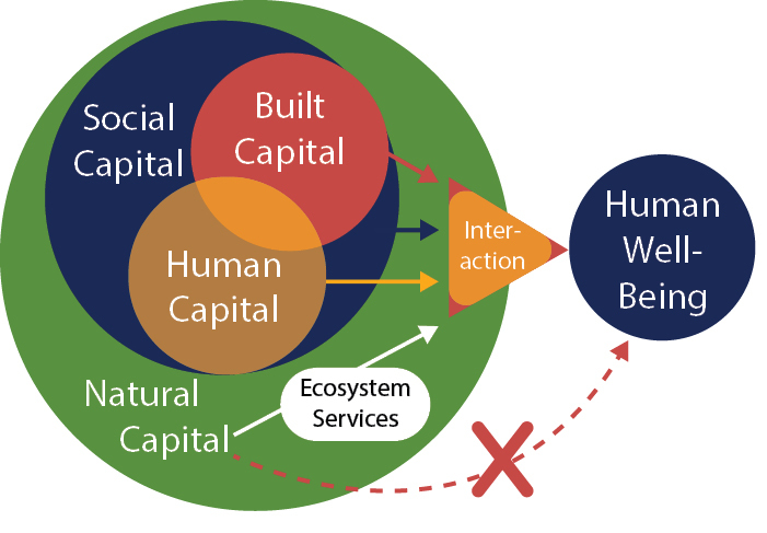
Biodiversity within the social-ecological system
Ecosystems and society are closely connected within a Social-Ecological-System (SES) (Chapter 2.3). The flow from the ecosystem towards society is generated through the supply of ES. The flow back into the system is society's influence on the ecosystem generated by drivers and governance. Each step within the system is related to biodiversity, which is the total stock or the living part of our natural capital. It determines the self-regulating capacity of the system and the attitudes of biodiversity dynamics, such as resilience or adaptability.
Within the system, specific ecological functions are essential to support and supply a specific ES: for example, primary production and pollination for food production, water infiltration capacity for water provision and organic decomposition for soil fertility. These specific functions depend upon a specific part of biodiversity and often, increasing biodiversity will optimise these functions.
Based on supply and demand, the final ES is generated, e.g. as a yield of food or wood, or a direct use of green infrastructure. Based on the benefits of a service, people will eventually value the components of biodiversity. This can be an ethical or 'intrinsic value', but also a cultural or instrumental value.
To complete the circle, the societal impact and the governance flow can be adjusted, which is based upon a biodiversity strategy. Here targets are formulated and adjusted on different scales. In line with these objectives, management plans will be developed and implemented and indicators will be chosen to measure the trend and to control the distance to the target.
Biodiversity and natural capital
Biodiversity as a whole is the 'living' part of the natural capital. It is our main capacity to generate ES and to ensure adaptation to environmental changes. Figure
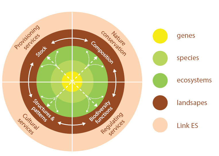
Four complementary perspectives of biodiversity, applicable to four organisation levels (gene, species, ecosystem & landscape).
To observe the dynamics of these biodiversity components, several indicator approaches are utilised. In most regions there is a dominance of 'composition' indicators linked with the nature conservation strategy while indicators for diversity of functions, connectivity or vegetation structure are rarely developed.
Biodiversity, ecosystem functions and services
Understanding how key ecosystem functions determine ES supply, how it depends on biodiversity and understanding the effects of shortcutting these functions by technological variants is crucial in the search for nature-based solutions. The basic interrelations between these components are sketched in Figure
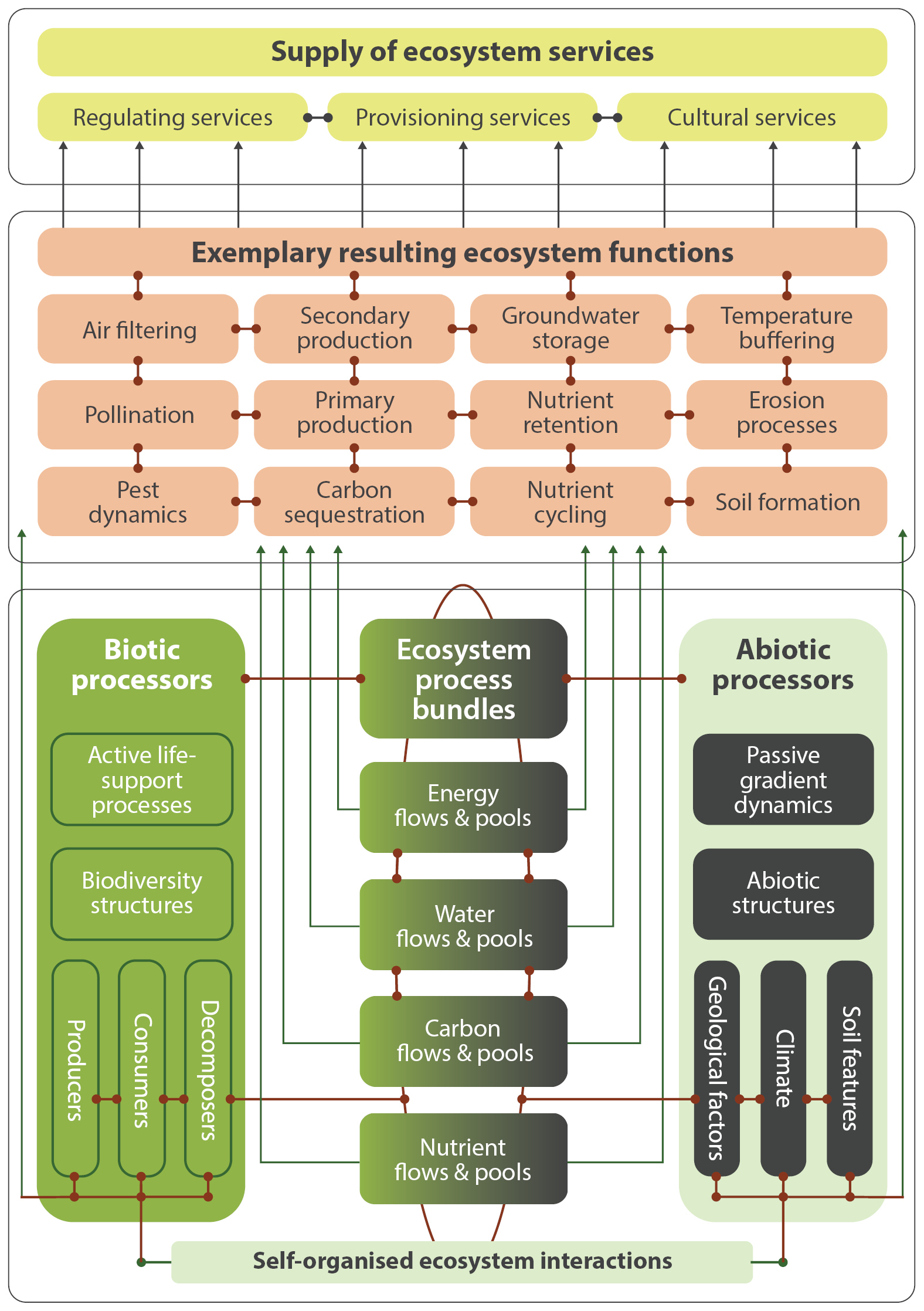
Diagram sketching the relations between ecological structures and processes (self-organised ecosystem interactions), exemplary ecosystem functions and ecosystem services. The interrelations are also described in the following Chapter 2.3.
Their characteristics can be aggregated into different groups of functional outcomes. To assess the overall state of these complex schemes, aggregated indicators such as ecosystem integrity or ecosystem health are developed. For instance, the indication of ecosystem integrity is based on an accessible number of structural items of biodiversity and ecosystem heterogeneity, combined with the functional items representative for the energy balance, the water balance and the matter balance of ecosystems.
The aggregation of functional units can also be made to represent specific ES. For example, photosynthesis leads to the fixation of CO2 which is influenced by the static abiotic site conditions, the dynamics of solar radiation, rainfall, evapo-transpiration or air temperature, but also by the nutrient and water provision and the state of competition with other plants. The result is an increase in phytomass and, on a longer time scale, an input of litter into the soil subsystem, where the carbon can be transferred and sequestered into long-term stable humic compounds.
These process sequences are interpreted as a functional subsystem, e.g. as carbon sequestration. These subsystems are illustrated by the middle box in Figure
Such connections are also responsible for most provisioning ES, because the primary and secondary production functions are strongly linked to the sequestration sequence. Also the regulation of nutrient budgets depends on the cycling and accumulating activities of the biotic system components, as well as the potential of the abiotic sphere to physically or chemically retain nutrients within the soil matrix. As a result of these process sequences, the seepage water is filtered and can be used for human purposes, e.g. as drinking water. Finally, cultural ES also depend on ecological interactions, because resulting ecosystem functions provide the basic preconditions to create and maintain certain structural conditions which human beings perceive as attractive phenomena.
As a result, we can observe very complex interrelations between ecosystem functions and ES. Some key functions and structures for 16 ES are listed in Table
Representation of ecosystem functions and structures steering (?) or supporting (?) an ecosystem service or a biodiversity target linked with intrinsic valuation. White fields demonstrate indirect effects.
|
Essential functions or structures for
the supply of a service |
Food
|
Wood production
|
Production energy crops
|
Venison
|
Water production
|
Pollination
|
Pest control
|
Preserving soil fertility
|
Flood control
|
Coastal Protection
|
Global climate regulation
|
Nutient regulation
|
Water regulation
|
Regulation air quality
|
Noise remidiation
|
Control erosion risk
|
Green space outdoor activities
|
Natura 2000
|
Green infrastructure
|
| Provisioning ES | Cultural ES | Nature conservation | |||||||||||||||||
| Primary production | |||||||||||||||||||
| Animal production | |||||||||||||||||||
| Soil formation | |||||||||||||||||||
| Nutrient availability / -cycling | |||||||||||||||||||
| Decomposition of organic material | |||||||||||||||||||
| Carbon storage | |||||||||||||||||||
| Conservation carbon stock | |||||||||||||||||||
| Storage rain water (infiltration capacity) | |||||||||||||||||||
| Ground water retention | |||||||||||||||||||
| Storage river water | |||||||||||||||||||
| River Drainage | |||||||||||||||||||
| Combating soil loss | |||||||||||||||||||
| Pollination | |||||||||||||||||||
| Pest control | |||||||||||||||||||
| Prevent disease | |||||||||||||||||||
| Air purification capacity | |||||||||||||||||||
| Scattering and absorption sound | |||||||||||||||||||
| Buffering coastal storms | |||||||||||||||||||
| Regulate population dynamics | |||||||||||||||||||
| Regulating ecosystem dynamics, succession | |||||||||||||||||||
| Stability ecosystem processes | |||||||||||||||||||
| Ecosystem resilience | |||||||||||||||||||
| Development of complex ecological networks | |||||||||||||||||||
| Develop ecosystem diversity / habitat quality | |||||||||||||||||||
But what is the role of biodiversity for each of those functions? Many experimental studies demonstrate that an increase in the variety of genes or species contributes to the optimisation of one of the functions. Sowing a grassland ecosystem with more species will, for example, generate a higher biomass. For wood biomass usually a positive diversity-production relationship is found, as a result of synergies between species and a better utilisation of resources, although some combinations create a negative effect due to competition. The fact that many functions are optimised by a higher biodiversity also means that a loss of diversity will generate a suboptimal function, often compensated by human inputs of energy, materials or technology (Chapter 5.1). It is a reality that technical compensation can lead to a disintegration of ES potentials and biodiversity in land use. For example, the correlation between species numbers and productivities is broken by the additional inputs of energy, manpower, fertilisers or pesticides. Thus, today, modern agriculture produces the highest biomass under conditions of (optimally) single-species monocultures.
Towards nature-based solutions
Each ES can be delivered in a gradient from naturally to technologically based solutions. Nature-based solutions depend more on biodiversity, generate a lower impact on surrounding ecosystems and guarantee a lower impact on other ES and a more sustainable use of the service itself. The use of a service is always a balance between supply and demand. In highly populated areas, for most ES the current demand is much higher than the supply. The excessive demand, together with a high drive for more human control, has affected and transformed most natural ecosystems towards the technological side of the gradient, in order to maximise a single service. The supporting and regulating role of biodiversity is systematically replaced by technological inputs, energy inputs, chemical inputs and management. This is true for nearly all provisioning ES, but also for most regulating and cultural ES. The challenge is to optimise the total supply of a bundle of ES, ensuring ES delivery and maintaining ecosystem functioning in the long term. Relying on more nature-based solutions will increase positive and decrease negative interactions.
Conclusions
All relationships in social-ecological-systems are driven by different aspects of biodiversity. All these interactions should be analysed in order to set up biodiversity strategies.
The creation of ES is founded on very complex schemes of ecological interactions with very high mutual interdependencies.
Understanding how key functions determine ES supply and how they depend on biodiversity and understanding the effect of short-cutting these functions by technological variants, is crucial in the search for nature-based solutions.
Moving towards more nature-based solutions of ES supply, generates positive effects for both biodiversity and the sustainable supply of ES bundles.
Further reading
- Cardinale BJ et al. (2012) Biodiversity Loss and Its Impact on Humanity. Nature 486(7401): 59-67.
- Haines-Young R, Potschin MP (2010) The links between biodiversity, ecosystem services and human well-being. In: Raffaelli D, Frid C (Eds.) : Ecosystem Ecology: A New Synthesis. BES Ecological Reviews Series, CUP, Cambridge, 110-139.
- Kandziora M, Burkhard B, Muller F (2013) Interactions of Ecosystem Properties, Ecosystem Integrity and Ecosystem Service Indicators - A Theoretical Matrix Exercise. Ecological Indicators 28 (SI): 54-78.
- Mace GM, Norris K, Fitter AH (2012) Biodiversity and Ecosystem Services: A Multilayered Relationship. Trends in Ecology & Evolution 27(1): 19-26.
- Morin X, Fahse L, Scherer-Lorenzen L, Bugmann H (2011) Tree Species Richness Promotes Productivity in Temperate Forests through Strong Complementarity between Species. Ecology Letters 14(12): 1211-19.
- Noss R F (1990) Indicators for monitoring biodiversity - a hierarchical approach. Conservation Biology 4: 355-364.
- Schneiders A, Van Landuyt W, Van Reeth W, Van Daele T (2012) Biodiversity and Ecosystem Services: Complementary Approaches for Ecosystem Management? Ecological Indicators 21: 123-33.
2.3. From nature to society
Linking people and nature: Socio-ecological systems
Although people have always depended on nature, in modern societies it is easy to lose sight of the fact that we still do. Indeed, many have argued that our failure to recognise the value of nature and especially the contribution that biodiversity makes to our well-being, explains much of our damaging behaviour towards the environment. It is against this background that the concept of ecosystem services (ES) is so important as it highlights the ways in which people and nature are connected.
The links between people and nature are, however, complex and so it is hardly surprising that people have defined ES in different ways. Some think of ES as the benefits that nature provides to people, like security and the basic material we need for a good life. Others view ES as the contributions that the ecosystem makes to such things. These differences in definition are explored in more detail in Chapter 2.4. For the moment it is sufficient to note that despite differences in the way ES are defined, most commentators agree that there is some kind of 'pathway' that goes from ecological structures and processes at one end through to the well-being of people at the other (Figure
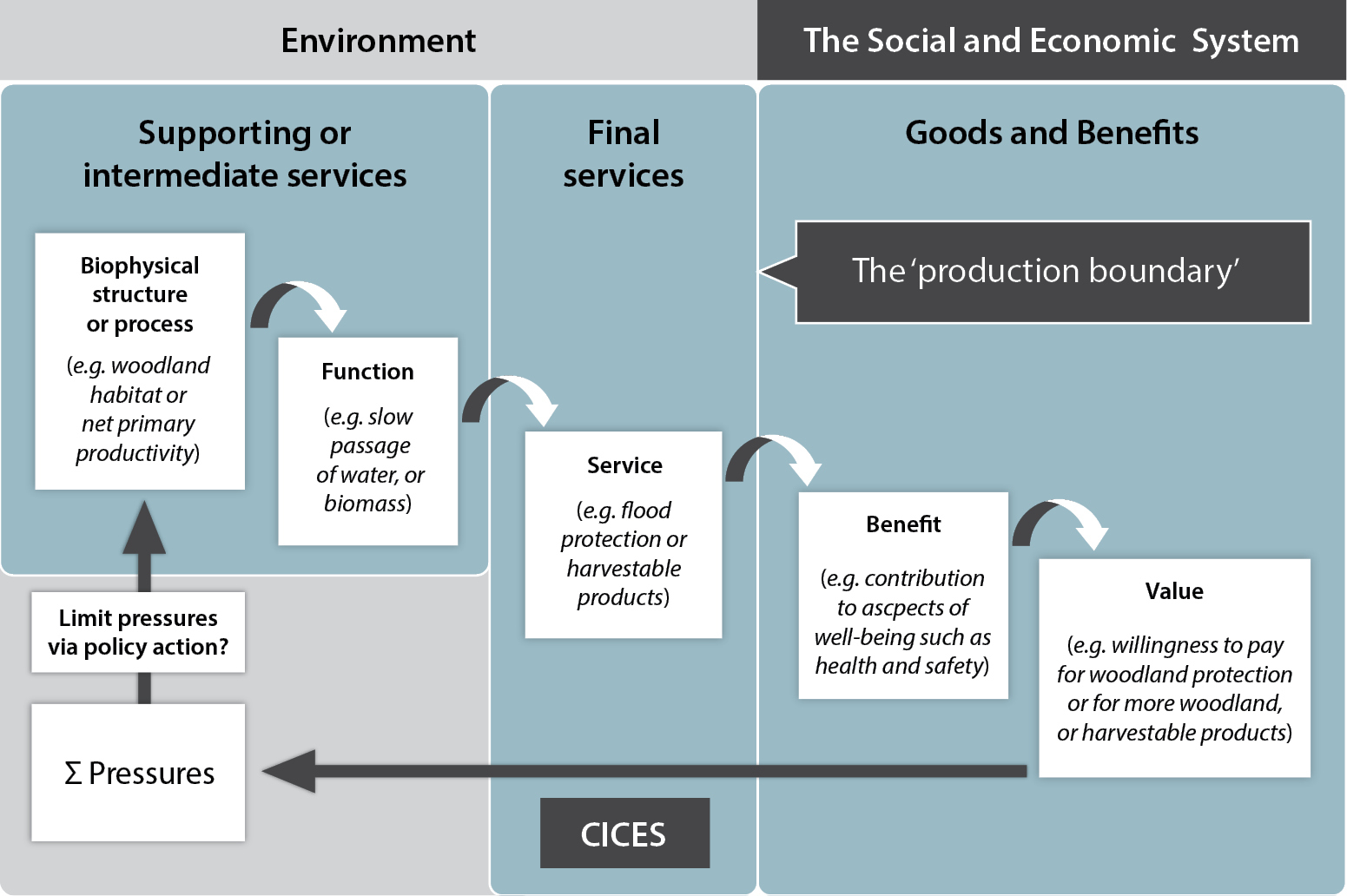
Note: 'CICES' in Figure 1 is the Common International Classification of Ecosystem Services, it is described in more detail in Chapter 2.4; it is a way of categorising and describing the final services that sit at the interface of nature and society.
Unpacking the cascade model
To understand how socio-ecological systems work, it is useful to 'unpack' the cascade model to see the inter-relationships between the elements. Ecosystem services are at the centre of the cascade model which seeks to show how the biophysical elements of the socio-ecological system are connected to the socio-economic ones; ES are at the interface between people and nature.
The 'ecosystem' is represented by the ecological structures and processes to the far left of the diagram. Often we simply use some label for a habitat type, such as woodland or grassland (Chapter 3.5), as a catch-all to denote this box, but there is no reason why we cannot also refer to ecological processes, such as 'primary productivity' as something that can also occupy this part of the diagram (Chapter 2.2). In either case, given the complexity of most ecosystems, when we want to start to understand how they benefit people, then it is helpful to start by identifying those properties and characteristics of the system that are potentially useful to people. This is where the idea of a 'function' enters into the discussion. In terms of the cascade model, these are taken to be the 'subset' characteristics or behaviours that an ecosystem has that determines or 'underpins' its capacity to deliver an ecosystem service. Some people call these underpinning elements 'supporting' and 'intermediate' services, depending on how closely connected they are to the final service outputs; we believe, however, this terminology deflects attention away from the important characteristics and behaviours of an ecosystem that generate different services. Thus using our terminology for one of the examples in Figure
In the cascade, it is envisaged that services contribute to human well-being through the benefits that they support; for example by improving the health and safety of people or by securing their livelihoods. Services are therefore the various ecosystem stocks and flows (Chapter 5.1) that directly contribute to some kind of benefit through human agency. The difference between a service and a benefit in the cascade model is that benefits are the things that people assign value to; they are therefore synonymous with 'goods' and 'products'. The cascade model suggests that it is on the basis of changes in the values of the benefits that people make judgements about the kinds of intervention they might make to protect or enhance the supply of ES; this is indicated by the feedback arrow at the base of the diagram. The importance of 'values' is that they can be expressed in many ways; for example, alongside monetary values, people can express the importance they attach to the benefits using moral, aesthetic and spiritual criteria (Chapter 4).
Despite the simplicity of the cascade model, it is useful in highlighting a defining characteristic of an ecosystem service, namely that they are, in some sense, final outputs from an ecosystem. They are 'final', in that they are still connected to the ecological structures and processes that gave rise to them and final in the sense that these links are broken or transformed through some human interaction necessary to realise a benefit. Often this intervention can take the form of some physical action such as harvesting the useful parts of a crop. The interaction might also be non-material and more passive involving, for example, the benefit obtained from the reduction or regulation of some kind of risk (flood risk is the example shown in Figure
Balancing supply and demand
Socio-ecological systems are, of course, more complex than Figure
Further reading
- Potschin M, Haines-Young R (2011) Ecosystem Services: Exploring a geographical perspective. Progress in Physical Geography 35(5): 575-594.
- Potschin M, Haines-Young R (2016) Defining and measuring ecosystem services. In: Potschin M, Haines-Young R, Fish R, Turner RK (Eds.) Routledge Handbook of Ecosystem Services. Routledge, London and New York, 25-44.
2.4. Categorisation systems: The classification challenge
Introduction
Categorising and describing ecosystem services (ES) is the basis of any attempt to measure, map or value them. It is the basis of being transparent in what we do, so that we can communicate our findings to others, or test what they conclude. So fundamental is the need to be clear about how we classify ES that it might seem that it is an issue that must already be well and truly resolved. The aim of this chapter is to suggest that this might not, in fact, be the case entirely and that the way we categorise ES is something that still represents a challenge.
A number of different typologies, or ways of classifying ES are available, including those used in the Millennium Ecosystem Assessment (MA) and The Economics of Ecosystems and Biodiversity (TEEB) and a number of national assessments, such as those in the UK, Germany and Spain. The problem with them is that they all approach the classification problem in different ways, involving different scale perspectives and different definitions resulting in the fact that they are not always easy to compare. In order to try to partly overcome this 'translation problem', the Common International Classification of Ecosystem Services (CICES) was proposed in 2009 and revised in 2013. A typology translator is available via the OpenNESS-HUGIN website".
We do not argue that it is better than any other system, but it illustrates the difficulty of designing a classification system that is simple and transparent to use. We will argue that the problem of classification is still worth working on - and it is certainly not something that can be taken for granted. We would encourage everyone to think about it when they embark on any kind of analysis involving ES.
The conclusion that we would like to advance is that the ES community probably needs to develop a number of different classifications or typologies that can be used to name and describe all the elements in the cascade that we described in Chapter 2.3, namely: the ecosystem or habitat units that give rise to the ES of interest, the ecological functions that are associated with them, as well as the benefits and beneficiaries whose well-being is dependent on the output of services and, of course, the values that people assign to these benefits. Services can also be classified according to such criteria as whether they give rise to private or public benefits, whether people can be prevented from accessing the service ('excludable' vs 'non-excludable'), or whether the use of a service by one individual or group affects the use by others ('rival' vs 'non-rival').
The Common International Classification of Ecosystem Services (CICES)
CICES was originally developed as part of the work on the System of integrated Environmental and Economic Accounting (SEEA) led by the United Nations Statistical Division (UNSD), but it has been used by the wider ecosystem services community to help define indicators of ES, or map them. In designing it, the intention was to provide a way of characterising 'final services', namely those that interface between ecosystems and society. In this sense, it follows the definition used in TEEB, namely that these final services are the things from which goods and benefits are derived. However, it did try to use as much of the terminology that was already widely employed and so used the categorisation of 'provisioning', 'regulating' and 'cultural' services that were made familiar by the MA.
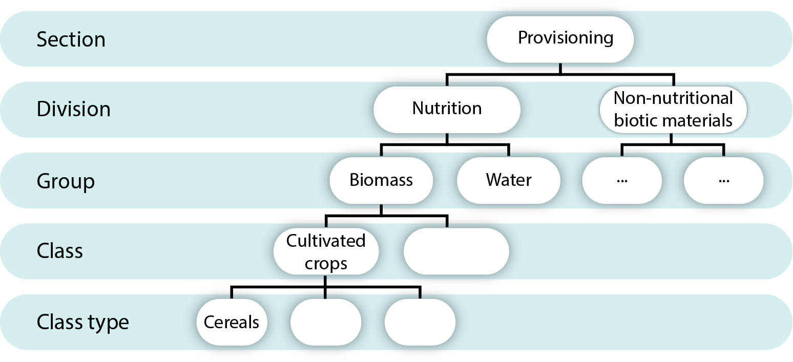
Material and energetic outputs from ecosystems from which goods and products are derived are contained in CICES provisioning services. Regulating services categories refer to all the ways that ecosystems can mediate the environment in which people live or depend on in some way and therefore benefit from them in terms of health or security, for example. Finally, the cultural category identified all the non-material characteristics of ecosystems that contribute to, or are important for people's mental or intellectual well-being. CICES is hierarchical in structure, splitting these major 'sections' successively into 'divisions', 'groups' and 'classes'. Figure
The full version of CICES is available online.
Facing the challenges of categorisation
The first challenge that working on CICES showed was how difficult it is to categorise 'final ecosystem services'. These, according to Boyd and Banzhaf, are the 'end-products of nature' who argue that it is important to define them clearly to avoid the problem of 'double counting' when we calculate their value; i.e. assessing the importance of a component of nature more than once generally because it is embedded in, or underpins, a range of different service outputs. More formally these authors suggest final services 'are components of nature, directly enjoyed, consumed, or used to yield human well-being'. The problem is that, what constitutes a final service, generally depends on the context in which the assessment or mapping exercise is being made; thus CICES lists potential final services.
A second challenge was whether abiotic ecosystem outputs like wind or hydropower, or minerals like salt, should be categorised as 'ecosystem services'. In the end, the argument that the category 'ecosystem services' should be restricted to those ecosystem outputs that were dependent on living processes won the day, because it strengthened arguments about the importance of 'biodiversity' to people; an accompanying provisional classification of abiotic services that follows the CICES logic has, however, been developed and is available.
It is worth mentioning that the final challenge which we encountered in designing CICES, was the difficulty that people have in distinguishing services and benefits. The distinction is a difficult one to make because it involves deciding where the 'end-product of nature' is transformed into a good, product or benefit, product or benefit as a result of human action of some kind. The distinction we use in CICES is whether the connection with the underlying ecological processes and structures is retained; hence the standing crop of wheat in the field is a final service from an agricultural ecosystem, but the grain in the silo is the good or benefit.
The distinction between services and benefits is an important one because a single service can give rise to multiple goods and benefits that all need to be identified if services are to be valued appropriately. In the case of rice for example, in addition to the harvest of the grain, rice straw and husks can be used for animal feed or as raw material for energy.
Using CICES - Taking stock
In this chapter we have used CICES to explore some of the challenges that we need to face when developing systems for categorising ES. These systems are complex and experience suggests that they will need to be developed in an iterative way, using experience to find out what works where and how naming conventions and definitions can be improved. While we have used CICES to illustrate some of these issues, it is important not to overlook the fact that it is a system that, despite limitations, has been used effectively.
For example, CICES forms part of the mapping framework designed to support the EU's Biodiversity Strategy to 2020 (the second report of the Mapping and Assessment of Ecosystem Services (MAES) uses CICES classes to identify a range of indicators that can be used for mapping and assessment purposes (see: http://biodiversity.europa.eu/maes/#ESTAB, accessed 30/01/2016; see also Chapter 7.1). A number of papers have appeared in peer-reviewed scientific literature that have either used CICES or commented upon it as part of their methodological discussion.
CICES has, for example, been used as the basis of the German TEEB study as well as the scoping work for a German National Ecosystem Assessment, NEA-DE. The TEEB report on Agriculture also recommends the use of CICES. Elsewhere, CICES has been refined at the most detailed class level to meet the requirements of ecosystem assessment in Belgium. Research in Finland used CICES to develop an indicator framework at the national scale. These kinds of applications suggest that the detailed class level in CICES can be useful as building block from broader reporting categories, the advantage being that these broader categories are themselves defined in a transparent way. These types of use illustrate the kinds of application that any good classification system must be able to support. Many more applications can be found - several are listed in the further reading material.
Outlook
While the applications of CICES suggest that the current framework is appropriate for many uses, it is also clear that we need to think carefully about how such systems can be developed. For example, researchers have suggest that it may need to be adapted to ensure that it is suitable for the assessment of marine and coastal ecosystems, or integrated more closely with typologies for describing underlying ecosystem functions. It is probable that marine interests were under-represented in the consultations that led to the current CICES version.
Thus while the current version of CICES clearly works for many purposes, given the importance of categorising ES in clear and transparent ways, the development of this and other systems needs to be reviewed constantly as our needs and concepts evolve. They are essential tools for our mapping and assessment work. It has been suggested, for example, that a classification, such as CICES, might form part of a more general systematic approach or 'blue print' for mapping and modelling ecosystem services. Other authors have emphasised that it is important to develop classification systems, such as CICES, that are 'geographically and hierarchically consistent' so that we can make comparisons between regions and integrate detailed local studies into a broader geographical understanding.
Our concluding point is that, whether CICES has a role to play or not, these kinds of systems will not build themselves. We need to be aware of the challenges that the categorisation of ES still poses and the fact that we have only just started to address them.
Note: At the time of writing, version 4.3 is to be used. This version is currently under revision and version 5 is under development. All details are available on the CICES webpage.
Further reading
- Boyd J, Banzhaf S (2007) What are ecosystem services? The need for standardized environmental accounting units. Ecological Economics 63: 616-626.
- Haines-Young R, Potschin M (2013) Common International Classification of Ecosystem Services (CICES), version 4.3. Report to the European Environment Agency EEA/BSS/07/007 (download: www.cices.eu).
- Potschin M, Haines-Young R (2016a) Defining and measuring ecosystem services. In: Potschin M, Haines-Young R, Fish R, Turner RK (Eds.) Routledge Handbook of Ecosystem Services. Routledge, London and New York, 25-44.
- Potschin M, Haines-Young R (2016b) Report on Workshop on "Customising CICES across member states". Milestone 19 of ESMERALDA (download at: http://www.esmeralda-project.eu/documents/).
Chapter 3. Background mapping
3.1. Basics of cartography
Introduction
Cartography (from Greek ?????? khartes, "map"; and ??????? graphein, "write") is the art and science of representing geographic data by geographical means. Maps are the main products of cartographic work and are graphic representations of features of an area of the Earth or of any other celestial body drawn to scale. Regardless of the map type or the mapping technique applied (Chapter 3.2), every map has a coordinate system, a projection, a scale and includes specific map elements. These attributes usually depend on the size and shape of the mapped geographical area and the graphical design of the map representation that needs to be informative and understandable for the map-user (Chapters 5.4 and 6.4).
Geographic Information Systems (GIS) are powerful tools for data Input, Management, Analysis and Presentation (IMAP principle) providing multiple possibilities for a better understanding of the structures and patterns of human and natural activities and phenomena (Chapter 3.4). Nevertheless, much of its easy-to-apply default-functionality can be misleading for an inexperienced map-maker.
In the present chapter, we discuss the main characteristics of maps such as coordinate system, geodetic datum, projection, scale and map elements; how to choose them accordingly and what their role is for proper use of a map. The use of GIS has significantly simplified mapping and provides a good environment for the visualisation of Ecosystem Services (ES).
Coordinate systems
The coordinate system of a dataset is used to define the positions of the mapped phenomena in space. It furthermore acts as a key to combine and integrate different datasets based on their location. This enables the performance of various integrated analytical operations, such as overlaying or merging data layers from different sources. Coordinate systems can be geographic, projected or vertical systems.
Geographic coordinate systems
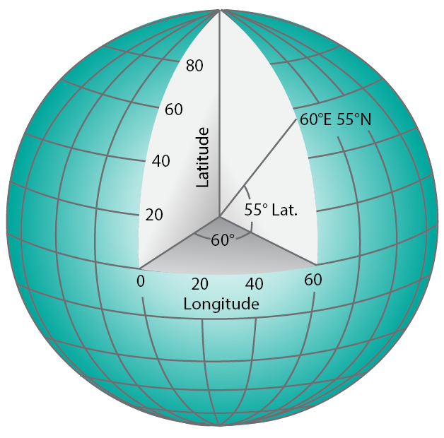
A Geographic Coordinate System (GCS) uses a three-dimensional spherical surface to define locations on the Earth, i.e. the Earth is represented as a sphere or a spheroid. A point on that sphere is referenced by its longitude and latitude values. Longitude and latitude are angles measured in degrees from the Earth's centre to a point on its surface. The Prime meridian and Equator act as reference for longitude and latitude respectively (Figure
Projected coordinate systems
A Projected Coordinate System (PCS) is based on a GCS that is transferred into a flat, two-dimensional surface. For that purpose, a PCS requires a map projection, which is defined by a set of projection parameters that customise the map projection for a particular location. The various map projections are discussed in detail below.
Vertical coordinate systems
A vertical coordinate system defines the vertical position of the dataset from a reference vertical position - usually its elevation (height) or depth from the sea level (Figure
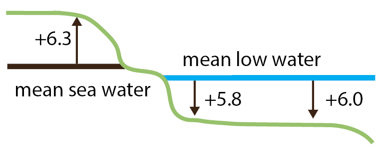
While the definition of a geographic or projected coordinate system is obligatory for all datasets, vertical coordinate systems are only needed if the vertical height of data is of relevance. Lack of, or wrongly defined, coordinate system information leads to problems of spatial data integration. (Figure
Therefore it is very important when using digital mapping tools that the used datasets are defined in an eligible coordinate system.
Geodetic datum and transformations
The geodetic datum defines a) the size and shape of the Earth and b) the orientation and origin of the used coordinate system through a set of constants. The geodetic datum can be based on flat, spherical or ellipsoidal Earth models:
- Flat Earth models are used over short distances so that the actual Earth curvature is insignificant (< 10 km);
- Spherical models represent the figure of the Earth as a sphere with a specified radius, leading to deformations in the model which are largest at the poles; used for short range navigation and global distance approximations; and
- Ellipsoidal models are the most accurate models of Earth; used for calculations over long distances; the reference ellipsoid is defined by semi-major (equatorial radius) and flattening (the relationship between equatorial and polar radii).
The ellipsoidal model can represent the topographical surface of the Earth (actual surface of the land and sea at some moment in time), the sea level (average level of the oceans), the gravity surface of the Earth (gravity model) or the Geoid. The Geoid is the equi-potential surface that the Earth's oceans would take due to the Earth's gravitation and rotation, neglecting all other influences such as winds, currents and tides.
The World Geodetic System 1984 (WGS-84) datum defines geoid heights for the entire Earth in a ten by ten degree grid. The Global Positioning System (GPS) is based on the WGS-84.
The geodetic datums can be horizontal (latitude and longitude), vertical (height) and complete. The transformation between datums requires the application of strict mathematical rules and sets of parameters, depending on the required transformation. Most GIS and mapping platforms support automated transformation between datums and coordinate systems.
Map projections
Map projections are mathematical representations of the Earth's spherical body on a plain surface through mathematical transformations from spherical (latitude, longitude) to Cartesian (x, y) coordinates. Map projections usually depend for the transformation on a form which can be developed or flattened - a plane, a cone, or a cylinder - which is attached to the sphere at one point or at one or two standard lines. The respective map projections are referred to as planar, conic and cylindrical (Figure
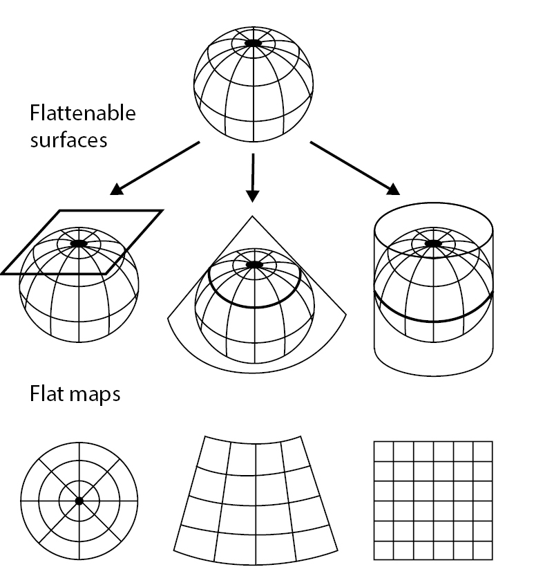
The transformation of a spherical surface into a plane leads to different distortions in the lengths, angles, shapes and areas of the mapped surface. The distortions are usually smallest along the standard lines and close to the attachment point. Depending on the shape and size of the mapped area, appropriate projection and standard lines should be selected. Distortions are inevitable and it is impossible to create the "perfectly" projected map that fulfils all map projection properties. The four properties of the map and their respective projection types are:
- Local shapes of the features on the map are the same as on the Earth's surface. This conformal projection maintains all angles.
- The areas of the features on the Earth are in the same proportions as on the map. Other properties - shape, angle, and distance - are distorted in equal-area projections.
- The scaled distances along the standard lines, or from the attachment point, to all other points on the map are maintained in equidistant projections. This is not valid along all lines or between any two points on a map.
- The directions on the map are correct in the true-direction (azimuthal) projection. It gives the directions (or azimuths) of all points on the map correctly with respect to the centre. Some true-direction projections are also conformal, equal-area, or equidistant.
For every map, only one or two of those properties can be fulfilled and the cartographer has to make a choice, depending on the purpose and needs of the map (see Chapter 5.4).
Scale
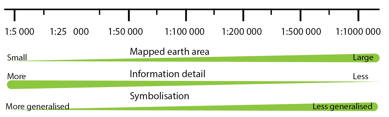
The scale represents the ratio of the distance between two points on the map to the corresponding distance on the ground. Thus large scale maps (with a large reciprocal value of the scale, such as 1:5,000) cover small areas with great detail and accuracy, while small scale maps (e.g. 1:1,000,000) cover larger areas in less detail (Figure
When choosing the map scale, the cartographer should consider:
- Purpose of the map - the mapped phenomena need to be well-represented in the selected scale;
- Map size - the scale need to be adapted to the size of the mapped area and the desired final size (format) of the map;
- Detail - the scale need to be adapted to the detail in which the phenomena are mapped.
Scale selection
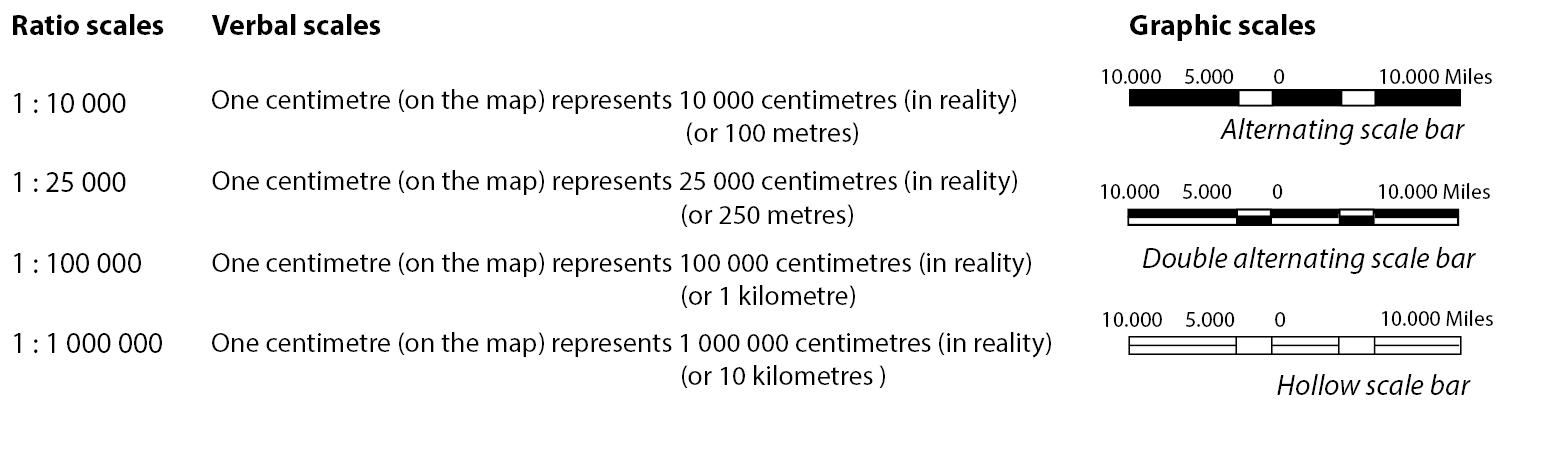
Map scales can be expressed as a ratio, a verbal statement or as a graphic (bar) scale (Figure
Elements of a map
Elements of a map are crucial for providing the map-user with critical information about the map content. Making a thematic map is to a large extent a creative act and the choice of map elements depends on the context, audience and the preferences of the map-maker. Nevertheless, there are three levels for representation of the elements of a map, presented here by by their level of relevance (Figure
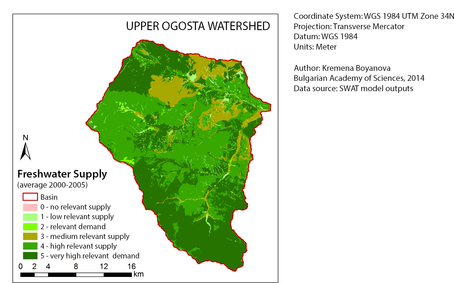
Example map and its elements: actual map, scale, north arrow, legend, title, coordinate system and projection, cartographer's name and institution, date of production, data source and neatline.
- Elements that make the proper reading of the map possible and it is recommended to add them to all maps:
- Scale information;
- Map direction - a symbol, usually an arrow, that indicates the true north (the direction to the North Pole); if a coordinate grid (graticule) is added to the map or on small-scale (e.g. continental) maps, a north arrow is not required;
- Legend - the legend lists all symbols, their sizes, patterns and colours used in the map and the features they depict (see Chapter 3.3); they should appear in the legend exactly as they are found in the body of the map;
- Elements that provide context:
- Title - should provide a short and clear statement about the map content, usually stating the name of the mapped area and the map theme (in ES maps - the mapped ES) along with the depicted year in thematic maps; it should be considered that this information can be included in the map legend title also;
- Projection - provides information about the projection and possible distortions in the area, distance, direction and shape of the mapped features;
- Cartographer's name and/or the authority responsible for the composition of the map;
- Date of production;
- Data sources used to create the map.
- Elements used selectively to assist effective communication (optional):
- Neatlines (clipping lines) - used to frame the map and indicate the exact area of the map;
- Locator maps - to place the body of the map within a larger geographical context;
- Inset map - a "zoomed in" map of small areas from the map with high relevance, where information is too clustered for the scale of the map body;
- Index maps - when labels or other information cannot be placed effectively in the body of the map, they can be input separately to increase readability.
Conclusions
Cartography is based on a long tradition and comprehensive knowledge of map-creation and map-use. ES map-makers still need to be aware of the general principles, techniques (Chapter 3.2) and logics (Chapter 3.3) of cartography, although with today's software programmes, it seems all too easy to create lots of maps rather quickly. Digital maps are the main means of map representation nowadays and the main tool for geographic data interpretation, visualisation and communication. They provide multiple opportunities but also 'traps' for the map-maker. Therefore, instead of producing large quantities of badly-compiled and misleading maps, ES map producers should harness the available knowledge and techniques in order to support the proper application of ES and ES mapping in science, decision making and society (Chapter 7).
Further reading
- Bugayevskiy LM, Snyder JP (1995) Map Projections - A Reference Manual. Taylor & Francis, Great Britain.
- Fenna D (2007) Cartographic Science: A Compendium of Map Projections, with Derivations. CRC Press, Boca Raton, Florida.
- International Hydrographic Bureau (2003) User's Handbook on Datum Transformations Involving WGS 84. 3rd Edition (Last correction August 2008). Special Publication No. 60. Monaco.
- Maling DH (1992) Coordinate Systems and Map Projections, 2nd Ed. Pergamon Press. Oxford.
- Monmonier M (1996) How to lie with maps. 2nd ed. The University of Chicago Press.
- Pearson F (1990) Map Projection: Theory and Applications. CRC Press, Boca Raton, Florida.
- Snyder JP (1987) Map Projections - A Working Manual. U.S. Geological Survey Professional Paper 1395. U.S. Government Printing Office. Washington, D.C.
- Snyder JP (1993) Flattening the Earth: Two Thousand Years of Map Projections. University of Chicago Press. Chicago, Illinois.
Online resources
ArcGIS (ESRI Desktop Help): http://resources.arcgis.com/en/help/
Buckley DJ (1997) The GIS Primer. Pacific Meridian Resources Inc.: http://planet.botany.uwc.ac.za/nisl/GIS/GIS_primer/index.htm
Further:
http://geokov.com/education/map-projection.aspx
http://www.progonos.com/furuti
http://www.colorado.edu/geography/gcraft/notes/mapproj/mapproj_f.html
http://www.colorado.edu/geography/gcraft/notes/cartocom/cartocom_ftoc.html
http://www.colorado.edu/geography/gcraft/notes/datum/datum_f.html
http://www.librry.arizona.edu/help/how/find/maps/scale
http://awsm-tools.com/geo/convert-datum
http://gitta.info/LayoutDesign/en/html/index.html
3.2. Mapping techniques
Introduction
Mapping is about the graphical representation of spatio-temporal phenomena. Illustrating our complex environment by symbols and graphics requires important decisions: Does the chosen map type properly reflect the Ecosystem Service(s) (ES) to be portrayed? Are more intuitive design choices available to visualise and explain a particular dataset? What happens if the map type does not fit the data? This chapter aims to investigate popular map types like dot maps, choropleth maps, proportional symbol maps, isarithmic maps and marker maps. We relate those types to inherent spatial and statistical characteristics of certain ES phenomena and give advice on advantages and possible pitfalls related to their usage.
Every ES map, whether paper or digital, is a graphical representation of ES in their geographic context. In most cases, such maps are built to facilitate understanding of ES in their spatial (Chapter 5.2) and/or temporal (Chapter 5.3) dimension. What kind of ES data should be presented to whom (e.g. general public, scientific community, ES-practitioners) greatly determine the mapping process: a process of abstraction from geographic reality to the final map. Scientific cartography developed an extensive body of theory and derived practical guidelines to accomplish this process. A major goal thereof is the provision of maps that can be intuitively read and correctly understood and used by the intended end user (Chapter 6.4).
Matching data and map type
Data are the result of measurements (Chapter 4.1), modelling (Chapter 4.4) or other quantifications (Chapter 4) of geographic phenomena. Air temperature data, for example, is typically gathered by taking measurements at several point locations. Data on tree diameters might look similar, since it uses the same geometry (points) and is measured on a metric level. However, the represented phenomenon (trees) is entirely different in nature, since trees only exist at discrete locations in space, while atmospheric conditions are continuously distributed and can be measured everywhere.
Different data models can be used to store, analyse and present spatial data, for example in Geographic Information Systems (GIS):
Vector data models represent discrete or continuous spatial phenomena by using points, lines and polygons. Vector data have high accuracy for displaying features with distinct boundaries; vector map data files usually use less memory capacity.
Raster data represent the world in a regular grid of cells (pixels). Raster models are often used for continuously varying phenomena or they are the result of remote sensing.
It is possible to convert vector to raster data and vice versa. However, based on the different data model concepts, such conversions normally lead to loss of information and/or data accuracy.
When defining maps as graphic representations with the aim of facilitating the understanding of spatial phenomena, mapping techniques that properly reflect their main spatial characteristics should be chosen. But what does properly reflect mean? According to the congruence principle from cognitive design, the structure and content of visualisations should correspond to the desired structure and content of mental representations. The basic mapping concept of scaling geographic space is appropriate in this respect, since distances and directions between entities are adequately represented by the scaled distances and directions of their corresponding map symbols (except when mapping on continental scale and projection distortion is apparent). Thus it facilitates the development of mental models on the respective spatial configuration. However, it makes a difference whether a spatially continuous geographic phenomenon like the air is represented as a set of discrete dots or by alternative graphic means corresponding better to its spatial continuity.
Spatial phenomena can be categorised based on spatial continuity and spatial (in)dependence. For each possible combination, Figure
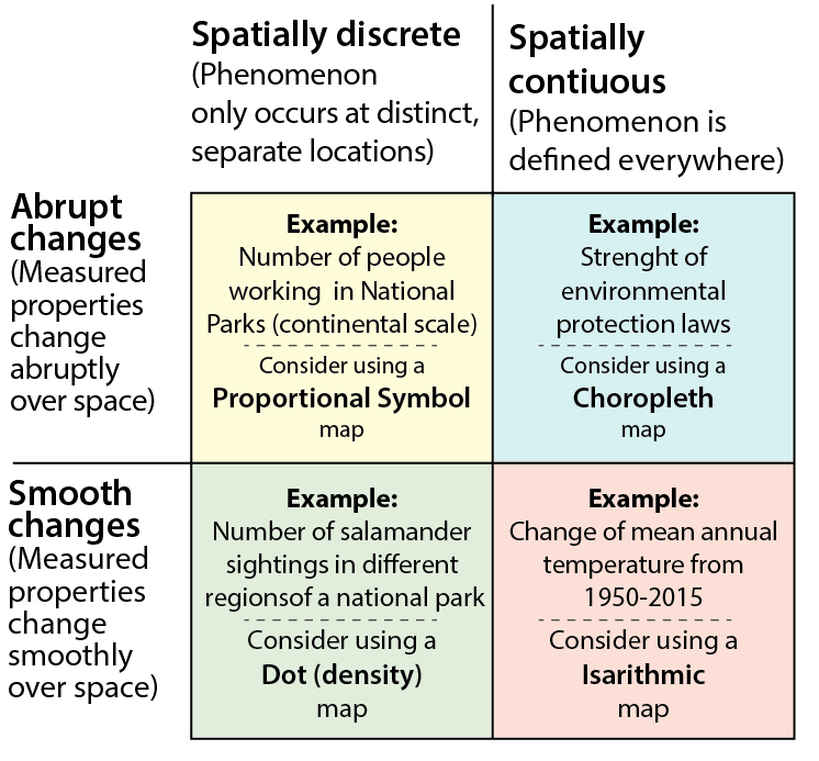
Models of geographic phenomena and suggested symbolisation methods. Simplified after
While such a scheme can assist in selecting an appropriate thematic mapping technique for quantitative data, there are further corresponding considerations:
What is the intended usage of the ES map (Chapter 5.4)? Does it merely act as an interface with the ES relevant entities, should it provide an overview on general spatial patterns or is it intended to allow for local comparisons?
Is the data related to individual locations or is it aggregated to enumeration units?
Is the data standardised (e.g. rates) or not (raw counts)?
The following section describes important thematic mapping techniques while addressing such considerations.
Mapping techniques
Common thematic mapping techniques include dot (density) maps, marker maps, choropleth maps, proportional symbol maps and isarithmic maps.
Dot (density) maps
In their simplest form of one-to-one feature correspondence, dot maps (also known as dot distribution maps) follow a very easy concept: at each location of the mapped entity, there is a corresponding small symbol in the map. Although this one-dot-per-feature approach is increasingly popular even in small scales and with very large numbers of features (http://demographics.coopercenter.org/DotMap/), dots quickly coalesce to a shading of variable intensity, which might be unfavourable for certain applications. In that case, a one-to-many approach is favourable, were each dot represents a fixed number of entities (e.g.: 1 dot = 100 people). The choice of the number of entities per dot is related to the chosen dot size, the scale and the density of feature locations. As a rule of thumb, points should start to coalesce in the map areas of maximum density.
Dot maps are especially suited to focus on the distribution patterns of entities or on differences in local densities. When using the dot density approach for polygonal aggregated data (e.g. number of people per district), the according number of points is placed within each polygon. To determine the position of each point within its polygon, several options apply:
- Random point distribution is straightforward and often used, although it might be misleading in cases with a very uneven distribution (e.g. randomly distributing points representing the population of Egypt on the country area).
- Adjust the point positioning within a polygon by using information on densities in neighbouring polygons.
- Use of ancillary information (e.g. settlement information from remote sensing data) for more precise point allocation.
Dot density maps which are based on aggregated data require absolute counts as a basis (e.g. number of persons per county). In addition, the use of an area-preserving map projection (see Chapter 3.1) is essential, since the density impression results from the number of dots per area unit on the map.
Heat maps are frequently seen derivatives of dot maps. Instead of showing the actual dots, they use areal colouring to represent their density. Dense areas get more reddish colours (therefore "heat") while areas with sparse data are normally coloured in blue. Although heat maps are quite popular, it is somewhat difficult to derive actual point feature numbers for a certain area.
Marker maps
Marker maps are a special form of dot maps that emerged with the advent of web mapping applications such as Google maps. Lying on top of a topographic base map, every marker or "pushpin" symbolises a feature of interest in its geographic location. With each marker being hyperlinked, the user can obtain additional object information or trigger certain actions, like booking a hotel room. The map itself acts foremost as an interface to data which is structured by its spatial location.
Paper maps showing the location of entities often use different symbols for different object types referenced in a legend. Thus the selection of the currently relevant object is performed visually by the user. Contrary to this, a web map allows the user to query the objects of interest within a database first and then show the query result in the map. Consequently, no further graphical differentiation of markers is necessary (but still possible).
Point markers are used to depict any type of feature geometry in the map, be it points, lines or areas. The main reason refraining from clickable areal symbols is explained by interaction challenges with other objects lying within the same area. Marker maps are often used to encode qualitative information. They mainly inform the user about individual locations and the spatial distribution pattern of the entities of interest. To prevent markers from coalescing in small scales, different mechanisms for grouping and/or selection can be applied.
Choropleth maps
Choropleth maps are preferably used to map data collected for areal units, such as states, census areas or eco-regions. Their main purpose is to provide an overview of quantitative spatial patterns across the area of interest. To construct a choropleth map, the data for each unit is aggregated into one value. According to their values, the areal units are typically grouped into classes and a colour is assigned to each class. This requires the use of meaningful colour-schemes (http://colorbrewer2.org) (Chapter 3.3), representing the sequential or diverging nature of the mapped phenomenon.
Although choropleth maps are very common, several pitfalls are inherently associated with them:
Variation within units is ignored, although the mapped phenomenon might vary considerably within (especially larger) units.
The boundaries between units often do not align with discontinuities in the mapped phenomenon. Especially the historically defined boundaries of administrative units often poorly align with spatial discontinuities of current social or natural processes (Chapter 5.2). Both problems, namely the variation within units and the definition of spatial boundaries apply for many ES and belong to the so called Modifiable Areal Unit Problem (MAUP; see Chapter 6.1).
Choropleth maps are only suitable for mapping standardised ("normalised") data like rates (yield per ha per year) or densities (persons per km?). Mapping absolute values (e.g. counts of persons per unit) is wrong since size differences of individual units will greatly affect the result: large units will tend to have higher values, small units lower ones. Even for experienced map users, it is impossible to mentally disentangle the resulting relationship between unit-size and colour for correcting the wrong impression of spatial distributions (compare Figure
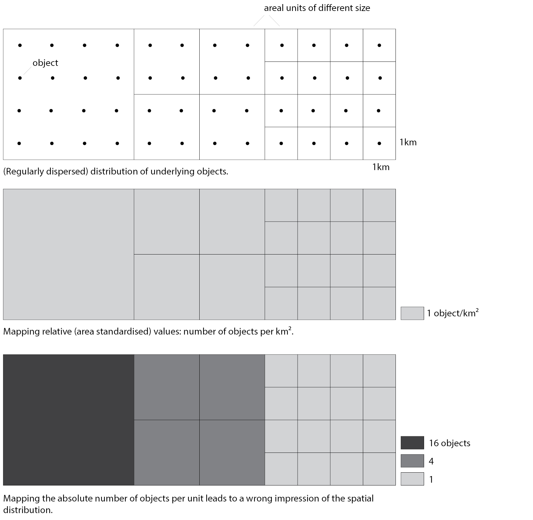
Only standardised data (rates etc.) should be mapped with choropleth maps. Inspired by
In summary, choropleth maps are a good choice to demonstrate standardised data aggregated to areal units, especially if there is little variation within units and the boundaries of the units are meaningful for the mapped phenomenon.
Proportional symbol maps
Based on our assumption that 'larger' means 'more', proportional symbol maps use variation in symbol size to depict quantities. While the size of point symbols can be used to denote quantitative attributes of point features (e.g. spring symbols scaled to water outputs), scaled point symbols are also used to represent data aggregated to areas, as discussed for choropleth maps. Contrary to the latter, not only is the colour of the areal units modified based on an attribute, but a point symbol is positioned within each area and the size of this symbol is scaled according to the desired attribute. Since comparing sizes is much easier than comparing shades, proportional symbol maps are especially effective for comparison tasks. According to the scheme in Figure
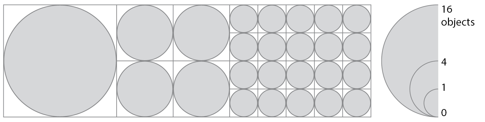
Symbol size relates well to the size of areal units, making proportional symbol maps capable of mapping non-standardised, absolute values (see Figure
In their basic form, the area of a symbol is scaled proportionally to the magnitude of the mapped attribute. However, several variants apply:
- Although the subject is controversial, perceptual scaling tries to adjust the symbol size to compensate the empirically tested tendency for underestimating the area of large symbols.
- The use of 3D-symbols like spheres or cubes allows scaling proportionally to symbol volume instead of area. Although volumes are estimated even more badly, this might be useful when large spans of data values have to be accommodated in the map.
- For data of extremely large or very small value ranges, data values might be classed and classes are assigned a set of 'graduated' symbols. While symbol sizes still represent the order of classes, symbols are not proportional to the magnitude of values any more. Thus additional information (e.g. in a legend) pointing to that fact is crucial for interpretation.
- At times, data is composed of several subgroups (e.g. total population by gender or age groups). To show this further subdivision, scaled diagrams can be used instead of plain symbols. Pie charts are often chosen due to their compactness.
Often, proportional or graduated symbols will overlap. While overall downscaling might be a solution, a small amount of overlap is acceptable. Using half-transparent, simple symbols like circles is a good strategy to cope with overlap as well. Web maps sometimes use cross-breeds of markers and proportional symbols: instead of permitting marker-overlap in small scales, nearby markers are aggregated into one symbol scaled to the number of markers it contains.
Isarithmic maps
Many ecosystem processes like climate regulation or air quality regulation take place in a spatially continuous manner. As a consequence, the related ES are also gradually varying over space. Isarithmic maps connect points of the same value (at certain intervals) by a line (=isoline) and are especially useful to map such smoothly changing 'continuous field' data. The most prominent examples of isolines are contour lines in topographic maps, connecting points of the same elevation. This concept can be used for all types of continuous fields. Isarithmic maps can be combined with areal colouring using continuous colour ramps. Alternatively, the areas between the isolines can be filled with a sequence of classed colours. A combination of isolines with analytical hill-shading intensifies the 'surface'-character of the mapped phenomenon.
The construction of isarithmic maps requires surface data, commonly modelled as point grid or Triangulated Irregular Network (TIN). Grounded on a base value and an interval, isolines are constructed from the field model using spatial interpolation. Using, for example, a base value of 50 and an interval of 100 to display a surface with values ranging between 54 and 320, isolines of the value 150 and 250 will be the result. Since isarithmic maps emphasise the continuous, smoothly varying character of a phenomenon, it is advisable to use them for such phenomena even though the data is being provided as discrete samples. As an example, data on ecological vulnerability based on districts could be considered: while each district might have assigned a value indicating its vulnerability, local vulnerability might smoothly change over space, independently of sharp district borders. Depending on the intended message ('objective representation of risk' versus 'hey governor, you are responsible for this highly vulnerable district, act!') it might make sense to create a continuous vulnerability surface from polygonal data and utilise an isarithmic map for its communication. When following such an approach, it is important to use only standardised (relative) values from enumeration units for surface generation. Methods like pycnophylactic interpolation or area-to-point kriging, guarantee that the overall volume remains constant while the surface is smoothed.
Apart from the basic thematic mapping concepts described so far, there are numerous other techniques: Cartograms, dasymetric maps, flow maps, animated maps or perspective views are just some examples for techniques meeting more specialised purposes.
Choosing an appropriate base map
A typical ES map consists of a topographic base map and one or more superimposed thematic layers showing the desired ES data. The base map provides the geographic reference to the ES data, informing the user on location while simultaneously providing a sense of the actual map scale. Depending on the used mapping framework mapping framework, there is often a choice between various base maps base maps. Some base maps can also be edited by the user to highlight or subdue certain object classes.
When choosing a base map, several aspects must be considered:
- Thematic support: The base map should support the thematic ES information; therefore it depends on the mapped ES topic, what kind of geographic features should be part of the base map. While some base maps focus on the street network street network, others emphasise the terrain or highlight administrative boundaries. Users should carefully think about what kind of information is required to support the mapped ES topic.
- Visual prominence: Base maps provide ancillary information, thus their place is in the visual background. In a digital context there are two common concepts to accomplish this: A dark base map with bright and saturated thematic information on top or a light and unsaturated base map overlaid by darker and more saturated thematic layers.
- Visual density: At each scale level, the base map should have approximately the same visual density (number of shown features per area). If the thematic ES layers are rather complex, a base map with a rather low visual density (e.g. only coastline and country boundaries) should be chosen.
Generalisation
Due to scale limitations it is not possible to show all spatial objects with all their detail in the limited map space. Generalisation aims to represent the ES-information in a level of detail appropriate for a given scale, user group and use context. It is necessary in cases where the visual density in maps is increasing rapidly, symbols overlap or topological conflicts become evident due to graphical scaling. Figure
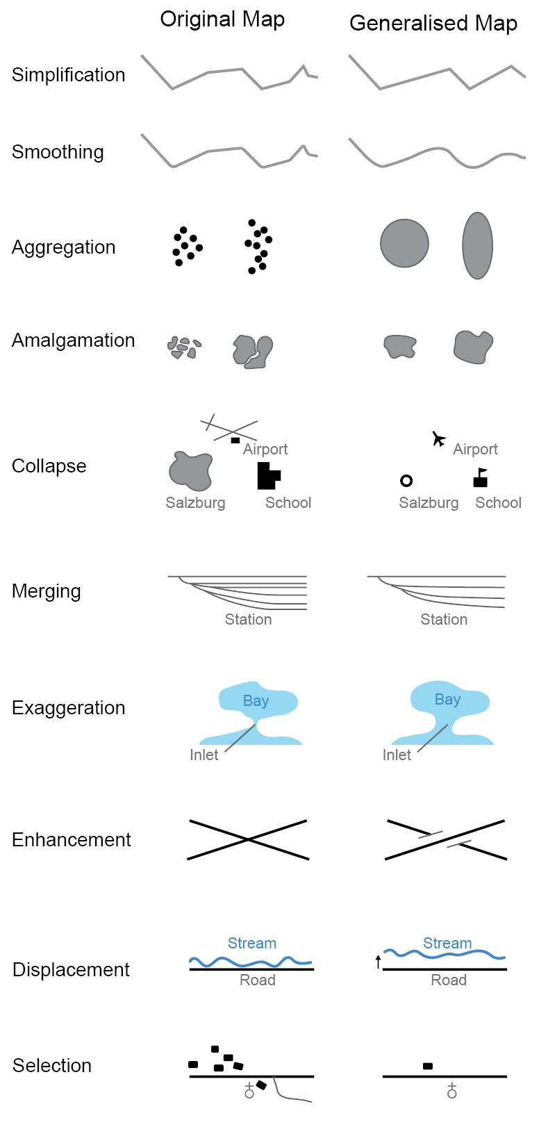
Conclusions
Map-makers can harness the broad knowledge base, experience and techniques available from cartography. ES-maps display highly complex human-environmental systems, consisting of discrete and continuous features. This complexity should also be respectively reflected in the maps, which need to be logical, clear, understandable and well-designed.
Further reading
- Brewer CA (1999) Colour Use Guidelines for Data Representation. Paper presented at the Proceedings of the Section on Statistical Graphics, Alexandria.
- Krygier J, Wood D (2011) Making Maps, Second Edition: A Visual Guide to Map Design for GIS: The Guilford Press.
- MacEachren AM (1992) Visualising uncertain information. Review of. Cartographic Perspectives (13):10-9.
- MacEachren AM (2004) How Maps Work - Representation, Visualisation and Design. 2 ed. New York, London: The Guilford Press.
- Muehlenhaus I (2013) Web cartography: map design for interactive and mobile devices: CRC Press.
- Slocum TA, McMaster RB, Kessler F, Howard HH (2009) Thematic Cartography and Geovisualisation. Clarke KC (Ed.) 3rd ed, Prentice-Hall Series in Geographic Information Science. Upper Saddle River, NJ: Pearson Prentice Hall.
- Tversky B (2005) Prolegomenon to scientific visualisations. In Visualisation in science education, Springer, 29-42.
3.3. Map semantics and syntactics
Introduction
Map-making and cartography combines science, arts, aesthetics and techniques that follow map-specific logic. Thus, cartography is strongly based on semiotics, the theory and study of signs and symbols. Map symbolisation is a key attribute of each map that determines the map elements (Chapter 3.1) and their applicability for communication (Chapter 6.4) and other uses (Chapter 7). Knowledge about basic semiotic principles is needed to produce proper ecosystem services (ES) maps that are fit for purpose.
Semiotics comprises semantics, syntactics and pragmatics:
- Semantics is the study of the relationships between signs and symbols and what they represent,
- Syntactics deal with the formal properties of languages and systems of symbols and
- Pragmatics analyse the relationships between signs and their users.
This chapter introduces map semantics and syntactics, which are the basis for the proper use of symbols, patterns and colours for different mapping purposes and scales. Chapter 6.4 deals with map pragmatics.
Graphic variables
Map features can be points, lines or areas (polygons). They are positioned on a map relating to their location in reality, the map scale and map projection (Chapter 3.1). Additional information is communicated by the choice of the map symbols' shapes, sizes, colour hues, colour values, colour intensities and textures. According to the different graphical variables' semantics, they are best used to show qualitative or/and quantitative differences. Most ES maps and ES model outputs (Chapter 4.4) are choropleth maps (Chapter 3.2) displaying areas of ES supply or demand. Some ES and landscape features are displayed as point or line features. Figure
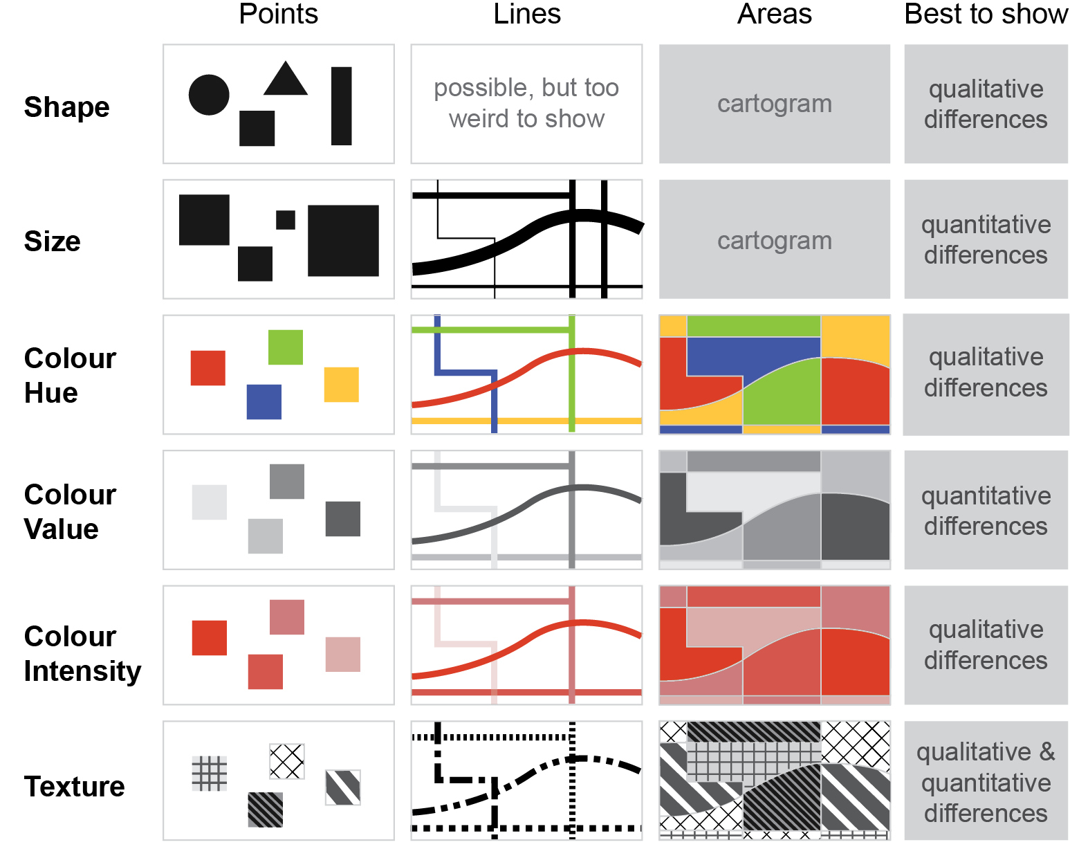
Shape
The map symbols' shapes are used to represent qualitative differences in thematic maps. In many cases, the shape is a logical connection to the feature that it represents (e.g. a petrol pump representing a gas station or a bed indicating a hotel). Text or respective letters/abbreviations are also often used (e.g. 'P' for car parking or 'H' for hotel). Shapes or adaptations of shapes are most often used for spatially discrete point features (see Chapter 3.2). They are rarely used for line features but can be applied in the form of cartograms (or anamorphic maps) for area features. In anamorphic maps, mapped areas are resized based on particular indicator values (see for examples: http://books.worldmapper.org).
Another relevant graphic feature that can be related to shape is orientation, which can be, for example, used to indicate directions of ES flows, movements or directional ES connections (Chapter 5.2). Topic-specific maps (e.g. geological map or weather maps) contain highly complex and specialised symbols. These maps often use their own logic of semantics and non-specialists can have difficulties interpreting them.
Size
Size is mainly applied in graphics to express quantitative differences, i.e. variations in amount or count (such as 'the more the larger' and, vice versa, 'the less the smaller'). Size can also be used to suppress less important features. The size of point and line features can be chosen accordingly, but following a rule of thumb to choose the difference in size according to quantitative differences in the features (e.g. double size for a double amount; see 'Classification of data' below). For graphical reasons, some smaller linear or point features (e.g. streams) are often enlarged, although the proportional size to other symbols might not represent reality (see 'generalisation' Chapter 3.2). The meaning of the different sizes (their semantics) should be explained in the map legend by providing the quantitative numbers that are behind the symbols (Chapter 3.1). Size variations of area features should refer to anamorphic maps or cartograms.
Combinations of different visual variables are possible, such as dot maps (see Chapter 3.2), illustrating distributions and densities by the symbols' shapes and quantities by their sizes. Depending on the scale of the map and the complexity of the landscape to display, shape and size may not offer sufficient detail or visibility for small symbols.
Colour hue, value and intensity
Colour hue is arguably the most powerful of the graphical variables. It can be applied to point, linear and area map elements. Different colour hues can relatively easily illustrate qualitative differences such as different land cover types in area maps. Variations in colour value or intensity are commonly used to portray quantitative differences in both dot and choropleth maps (see Chapter 3.2).
When using colour in maps, the map-maker needs to be aware that the different colours have specific meanings for many people and cause different psychological effects when viewed. Figure
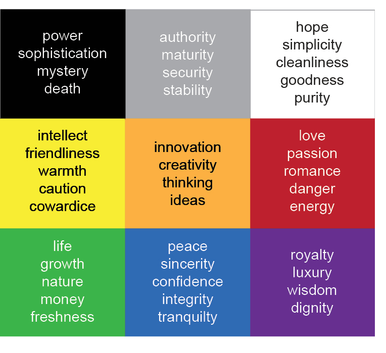
Possible psychological associations of different colours for viewers (based on: http://guity-novin.blogspot.de/2014/07/chapter-70-history-of-color-color-wheel.html).
Due to the omnipresent nature of mapping products in all kinds of media, the map-maker needs to be aware that many colours are connected with particular geographic phenomena (e.g. green for forests, blue for water bodies, red or black for urban areas; see for example the European CORINE land cover data set). Applying such commonly used colour schemes is essential for an easy and correct communication of the map content (see Chapter 6.4).
Texture
Texture can efficiently illustrate qualitative differences, for example different soil types, land uses or hydrological units. Similar to colour hue, texture can be applied for point, linear and area map features (see Figure
Classification of data
The normal map-user has a limited capacity to differentiate between a large number of colour (or grey) values or intensities. Therefore it is often necessary to classify (group) quantitative data that are to be portrayed in the thematic map. A small amount of graphic variations then appears in the map based on the reduced number of pre-defined data classes. Aggregating of map features into appropriately-defined classes increases the readability and the usefulness of the map. Distribution patterns in the landscape can be identified easier. The choice of the appropriate data classification method and the number of classes has a significant bearing on the quality of the final map. Data classification should be carried out carefully and with consideration to the data distribution and the purpose of the map. The data distribution can be checked by using histograms (Figure
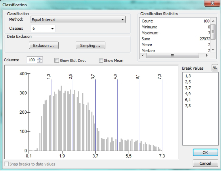
The most common data classification methods are:
- Equal intervals,
- Quantiles,
- Natural breaks (Jenks),
- Geometric intervals and
- Standard deviations.
GIS or cartography software programmes (see Chapter 3.4) normally offer algorithms and standardised procedures for classification of data (Figure
Equal intervals
The data are divided into equal-sized intervals (such as an interval of 2, resulting in the classes 0-2; 2-4; 4-6; etc.). To avoid double-representation of data, each subsequent class must start with the next higher value than the one before ended (i.e. 0-2; 2.1-4; 4.1-6 etc.) (cp. Figure
Quantiles
When using quantiles, all available data values are divided into unequal-sized intervals so that the number of values is the same in each class. Different from the equal interval method, each class (including the extremes) have the same number of values. This often leads to maps with more classes portraying the middle value ranges. The map-user has to be aware of the classification method and carefully check the map legend when reading the map.
Natural breaks (Jenks)
The natural breaks classification method is applied by checking the data distribution (for example in a histogram or in a graph) and placing class breaks around data clusters. This avoids large value variations within one class and highlights differences between different classes. As with quantile-based classified maps, the map-creator and reader must be aware of the effects of this (sometimes subjective) data classification on the resulting map.
Figure
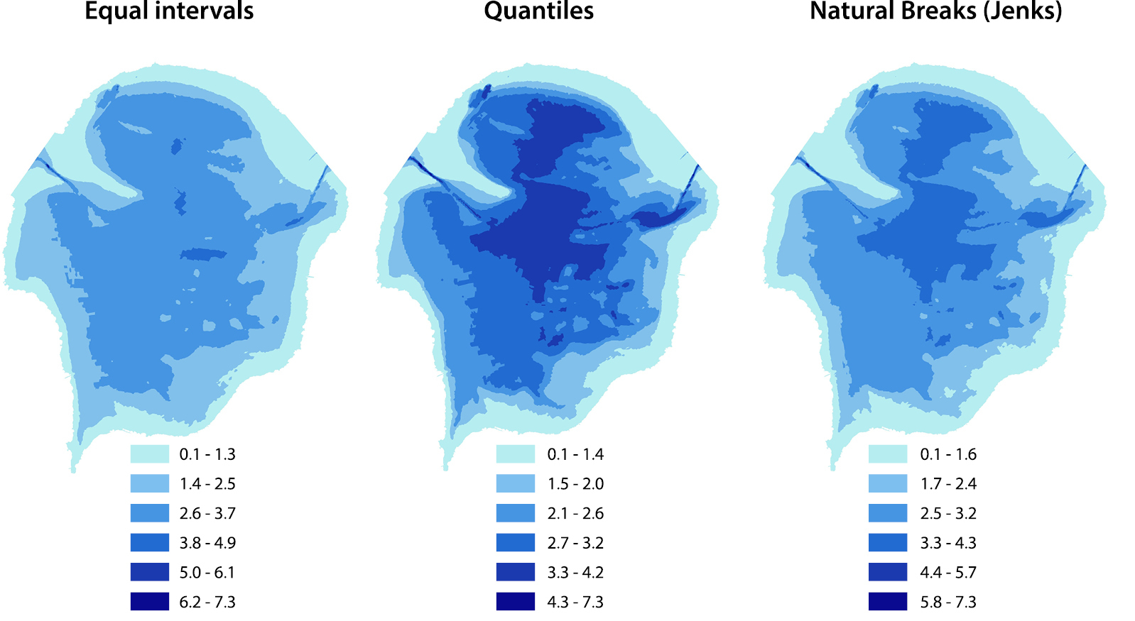
Common mistakes
An inappropriate selection and application of graphic variables or the wrong data classification method can lead to map misinterpretation (Chapter 6.4), confusion or production of poor map products. Bad choice of colours, the most powerful graphic variable, can render a map useless.
A common mistake, which has been heavily stimulated by the seemingly easy map-creation with various GIS, cartography and presentation software programmes, is the choice of too vibrant colour ramps that combine contrasting hues and go across for example red-blue-orange-green-yellow-brown colour schemes ignoring effects that different colours have on the map-user. Most map users may not be able to differentiate more than six or eight different colours within one map, depending on the map's complexity and the size of the depicted symbols. This number may be lower for people with limited colour vision. Another important consideration when creating colour maps is that colours are not recognisable if the map is reproduced in black and white or greyscale. Even if printed in colour, mismatches can occur between the printed version and the computer screen if different colour models are used.
Using bad map symbols that do not follow the logics of map semantics, syntactics and pragmatics often leads to noises in the map- maker/map-user communication (map coding; Chapter 6.4). Different cultural, societal or educational backgrounds may lead to different interpretations of symbols. A cartographer or a trained map-user will interpret a map differently from a novice map user.
Another common mapping mistake relates to the Modifiable Areal Unit Problem (MAUP; see Chapters 3.2 and 6.1). MAUP becomes especially relevant when using different colour values or intensities in choropleth maps. Additionally, the use and combination of too many different colours, patterns and symbols hamper easy and appropriate map comprehension by giving the map a 'nervous' look. Maps that are overcharged with information might run the risk of being ignored.
The map-maker needs to be aware of the finite capacity of the map-user to differentiate between the various graphic variables, especially in complex maps covering large spatial scales (Chapter 5.7). The appropriate classification of quantitative data is therefore a very important step in thematic map compilation.
Solutions
When choosing from the different graphic variables shape, size, colour hue, value, intensity and texture presented above, the map-maker needs to be aware of the semantics and syntactics relevant to the choices. The semantic and psychological effects of different colours should therefore be carefully considered and maps should not be overloaded with too many different colours. When illustrating quantitative differences, the colour ramp should only have one or two colour hues (Figure

It is also advisable to check the visibility of the selected colours after printing in black and white. Texture may be a better choice than colour hue or intensity to portray different classes in black and white maps.
Regional peculiarities need to be taken into account when compiling ES maps because of the trans-disciplinary and complex nature of ES. Involving stakeholders and harnessing their local or subject-specific knowledge can help to avoid cultural traps or misinterpretations. A stepwise process that seeks feedback from stakeholders and map-users can help to improve maps and reduce the number of map misinterpretations.
A proper map legend showing all symbols, symbol sizes, colour hues, values, intensities and orientations that appear in the map is mandatory in each map in order to read the map accordingly (see Chapter 3.1). Text in maps, where useful and appropriate, can support the information given by the map symbols. It must be legible, easy to comprehend and in the language of the map-user.
Specifics of ecosystem service maps
ES science involves several scientific disciplines and links multiple topics and quantification methods (Chapter 4) at various spatial and temporal scales (Chapter 5.7). Therefore ES mapping includes several challenges (see Chapter 3.7), that can be related to map semantics and syntactics.
The six key graphical variables described above are also applied in ES maps, depending on the ES to be displayed, what has to be mapped (Chapter 5.1), where (Chapter 5.2), when (Chapter 5.3) and why (Chapter 5.4). Many regulating ES (Chapter 5.5.1) can, for example, be related to natural phenomena which are often indicated by the choice of texture or orientation (e.g. for flows). Different intensities are depicted with appropriate colour hues. Provisioning ES maps (Chapter 5.5.2) often display service providing areas (Chapter 5.2), which can be point units (graphical shape) or area units (mostly displayed in choropleth maps; see Chapter 3.2). Quantities of ES supply can be portrayed by size variations (point sources, linear flows) and gradational colour values, intensities or textures. Cultural ES (Chapter 5.5.3) can be related to spatially discrete point features (e.g. iconic landmarks or religious sites displayed by map symbol shape variations) or more continuous area features (aesthetic experience based on viewsheds or landscape setting displayed by area features).
Conclusions
The map-makers have to take responsibility for their products as it is easy to impress or mislead map-users with colourful and attractive maps. ES maps are of high political, societal and economic relevance (Chapter 7). Therefore their compilation should closely follow the logics and the well-founded knowledge from graphic semiology. Based on the diversity of ES map-makers, map-users, the complex topics to be displayed and their high societal relevance, ES maps need to be designed with care. Well-constructed maps can properly communicate and explain complex ES phenomena.
Further reading
- Bertin J (1967) Semiologie Graphique. Les diagrammes, les reseaux, les cartes. With Marc Barbut [et al.]. Paris: Gauthier-Villars. (Translation 1983. Semiology of Graphics by William J. Berg).
- Dent B, Torguson J, Hodler T (2008) Cartography: Thematic Map Design. 6th edition. McGraw-Hill Science/Engineering/Math.
- Monmonier M (1996) How to lie with maps. 2nd ed. The University of Chicago Press.
- Muehrcke PC (2005) Map Use: Reading, Analysis, and Interpretation. 5th ed. J P Pubns.
- Wood D (1992) The Power of Maps. The Guilford Press.
3.4. Tools for mapping ecosystem services
Background
Mapping tools have evolved impressively in recent decades. From early computerised mapping techniques to current cloud-based mapping approaches, we have witnessed a technological evolution that has facilitated the democratisation of Geographic Information Systems (GIS). These advances have impacted multiple disciplines including ecosystem service (ES) mapping. The information that feeds different mapping tools is also increasingly accessible and complex. In this chapter, we review the evolution of mapping tools that are shaping the field of ES mapping together with the different sources of information that exist at this point. We discuss briefly the suitability of these approaches for mapping different ES types and for different scientific and policy aims. Finally, we elaborate on the integration of multiple tools (from desktop applications to sensor, web-based, or mobile devices) and on the future developments of these methods and the possibilities they may open for ES mapping.
Introduction
ES mapping has achieved rapid progress in a very short time frame. To our knowledge, the first peer-reviewed ecosystem service maps were published in 1996 and, since then, a large number of ad hoc mapping studies have been conducted and a variety of tools have been developed to systematise ES mapping. The progress we have witnessed corresponds to advances in computing power, modelling and GIS, the recognition of a plurality of ES approaches (i.e., participatory mapping (Chapter 5.6.2) and biophysical modelling (Chapters 4.1 and 4.4), and the consensus that ES maps provide a direct connection between ES and the landscape and therefore with policy (Chapter 7.1).
Description of main mapping software, tools and databases
Computing power and data availability that support GIS analysis have evolved substantially in recent years. Several freeware GIS platforms have been developed, such as QGIS (Quantum GIS), GRASS GIS (Geographic Resources Analysis Support System GIS), SAGA (System for Automated Geoscientific Analyses), and gvSIG (Generalitat Valenciana Sistema de Informacion Geografica) that provide similar functionality to the popular commercial ArcGIS software from ESRI (a list of GIS software is available here).
Specific modelling approaches for mapping ES have been developed by different institutions worldwide, resulting in a wide variety of possibilities for ES analysts' use (Table
List of the most common ES mapping tools.
| Tool | Platform | Scale2 | Source |
|---|---|---|---|
| Integrated Valuation of Ecosystem Services and Tradeoffs (InVEST) | ArcGIS/Stand-alone | Municipal to provincial | http://www.naturalcapitalproject.org/invest/ |
| Artificial Intelligence for Ecosystem Services (ARIES) | Graphical User Interface (GUI)/Web-based | Municipal to provincial | http://aries.integratedmodelling.org/ |
| Multiscale Integrated Models of Ecosystem Services (MIMES) | Simile software | Village/farm to global | http://www.afordablefutures.com/orientation-to-what-we-do/services/mimes |
| Social Values for Ecosystem Services (Solves) | ArcGIS | Municipal to provincial | http://solves.cr.usgs.gov/ |
| Land Utilisation Capability Indicator (LUCI) | ArcGIS | Village/farm to provincial | http://www.lucitools.org/ |
| Integrated Model to Assess the Global Environment (IMAGE) | Set of models | Global | http://themasites.pbl.nl/models/image/index.php/Welcome_to_IMAGE_3.0_Documentation |
| Co$ting Nature | Web-based, Google Earth | Municipal to provincial | http://www.policysupport.org/costingnature |
| Ecosystem Valuation Toolkit | Web-based | Municipal to provincial | http://esvaluation.org/ |
| ESM-App | Android Smartphone app | Municipal to provincial | http://www.ufz.de/index.php?en=33303 |
The use of GIS in ES mapping can take three general approaches: (1) analysis tools built into GIS software packages; (2) disciplinary biophysical models applied for ES assessment (e.g., hydrological models such as the Soil and Water Assessment Tool, SWAT or Variable Infiltration Capacity model, VIC for water-related ES); and (3) integrated modelling tools designed specifically for ES assessment (e.g., InVEST, ARIES). The first approach is applicable for simple land cover-based analyses and indicator-based ES mapping (see Chapter 5.6.4) that have been used for example in Mapping and Assessment of Ecosystems and their Services (MAES). The second approach is appropriate for more complex model-based analyses of services that integrate expertise from specific disciplines (e.g., ecology for crop pollination or hydrology for flood regulation mapping). The third approach extends the second one by utilising modelling tools that can assess trade-offs and scenarios for multiple services.
Several ecosystem service valuation databases have been developed as well, such as The Economics of Ecosystems and Biodiversity (TEEB) Valuation Database and the Ecosystem Valuation Toolkit and these might be used to create ES maps. The Ecosystem Services Partnership (ESP) Visualisation Tool is a database consisting of ES maps prepared by different researchers intended to promote synthesis of mapping studies (see chapter 7.9).
Applicability of mapping tools
In-depth assessment of the different mapping tools is necessary to understand which one will best fit the user?s ES mapping context: time and data availability, mapping skills, types of services to map, accuracy required, expected impact in decision-making and overall study aims. This means that no tool fits all criteria perfectly. Some highly complex models can provide policy support in regions with considerable time, data and personnel resources. Other approaches exist that allow ES to be mapped with more limited budgets and shorter time frames. The intended use of the maps (i.e., for raising awareness or direct use in policy-making) will also influence the decision on which tools to use (see Chapter 5.6.1).
In many cases, the type of ES under assessment will determine the mapping approach or tools to use. Services such as water regulation usually require modelling approaches that integrate meteorological databases, vegetation, soils and topographic data (Chapter 5.5.1), while others such as cultural identity might require a participatory mapping approach (Chapters 5.5.3 and 5.6.2). Other services such as food production might use complex agricultural models or indicator-based approaches (Chapter 5.5.2). However, the complex nature of ES and the inter-linkages between provisioning, regulating and cultural services have led to the use of different tools for each ecosystem service.
It is also important to consider how different mapping tools account for accuracy, reliability and uncertainty. Accuracy is established through successful calibration, reliability through successful application in different contexts and uncertainty through methods that estimate and transparently communicate uncertainty. These aspects have not been adequately covered in the past and still need to be developed for several tools. Greater transparency in the presentation of results and associated uncertainties (Chapter 6) is needed so that informed decisions can be made about the extent to which ES maps can be used for different purposes and which tools are best applied in different contexts and locations.
Future developments
Several challenges lie ahead for mapping ES. These are related to the progress that is currently underway in research and monitoring, remote sensing, sensor networks, data storage, data and knowledge integration, data harmonisation and sharing, database and tool maintenance and crowdsourcing, among others.
On the technical side, the accumulation of a growing quantity of data raises the challenge of effective storage and analysis of large amounts of data and is leading to an increased emphasis on machine learning, pattern recognition (in complex data or remote sensing products), and data mining. Initially high data storage requirements were addressed by large data storage and supercomputer facilities, but falling costs of distributed solutions have pushed computing towards scalable clusters of computers, grids and cloud computing, all aimed at increasing demand-driven computational power. Some ES modelling approaches using grids include: Tropical Ecology Assessment and Monitoring (TEAM) Network, Web-based Data Access and Analysis Environments for Ecosystem Services, ARIES, enviroGRIDS and biodiversity virtual e-laboratory (BioVel). The advantage of grids/clouds is that they are on-demand, self-service approaches, so the user can unilaterally obtain the necessary computing capabilities, such as server time and network storage, without having to interact with each service's provider. Cloud-based modelling tools and interfaces (e.g., OpenMI) will enable the joint development of and access to modelling and visualisation tools.
The ongoing development and maintenance of ES mapping tools (including free open-source software) require adequate funding. Further integration of ES mapping tools with policy will contribute to ongoing developments in the field and a tailored approach towards decision-making aims.
Disclaimer
Any use of trade, product, or firm names is for descriptive purposes only and does not imply endorsement by the U.S. or any other Government or by the authors of this article.
Further reading
- Bagstad KJ, Semmens DJ, Waage S, Winthrop R (2013) A comparative assessment of decision-support tools for ecosystem services quantification and valuation. Ecosystem Services 5: 27-39.
- Bagstad KJ, Reed JM, Semmens DJ, Sherrouse BC, Troy A (2015) Linking biophysical models and public preferences for ecosystem service assessments: a case study for the Southern Rocky Mountains. Regional Environmental Change: 1-14.
- Bateman IJ, Jones AP, Lovett AA, Lake IR, Day BH (2002) Applying Geographical Information Systems (GIS) to environmental and resource economics. Environmental & Resource Economics 22: 219-269.
- Crossman ND, Burkhard B, Nedkov S, Willemen L, Petz K, Palomo I, Drakou E, Martin-Lopez B, McPhearson T, Boyanova K, Alkemade R, Egoh B, Dunbar MB, Maes J (2013) A blueprint for mapping and modelling ecosystem services. Ecosystem Services 4: 4-14.
- Drakou EG, Crossman ND, Willemen L, Burkhard B, Palomo I, Maes J, Peedell S (2015) A visualization and data-sharing tool for ecosystem service maps: Lessons learnt, challenges and the way forward. Ecosystem Services 13: 134-140.
- Eade JDO, Moran D (1996) Spatial economic valuation: Benefits transfer using geographical information systems. Journal of Environmental Management 48: 97-110.
- Klug H, Kmoch A (2015) Operationalizing environmental indicators for real time multi-purpose decision making and action support. Ecological Modelling 295: 66-74.
- Malinga A, Gordon L, Jewitt G, Lindborg R (2015) Mapping ecosystem services across scales and continents - a review. Ecosystem Services 13: 57-63.
- Nelson E, Mendoza G, Regetz J, Polasky S, Tallis H, Cameron RD, Chan KMA, Daily GC, Goldstein J, Kareiva PM, Lonsdorf E, Naidoo R, Ricketts TH, Shaw RM (2009) Modeling multiple ecosystem services, biodiversity conservation, commodity production and tradeoffs at landscape scales. Frontiers in Ecology and the Environment 7(1): 4-11.
- Schroter M, Remme RP, Sumarga E, Barton DN, Hein L (2015) Lessons learned for spatial modelling of ecosystem services in support of ecosystem accounting. Ecosystem Services 13: 64-69.
- Stoll S, Frenzel M, Burkhard B, Adamescu M, Augustaitis A, Bae?ler C et al. (2015) Assessment of ecosystem integrity and service gradients across Europe using the LTER Europe network. Ecological Modelling 295: 75-87.
3.5. Mapping ecosystem types and conditions
Introduction
Ecosystems are defined by the UN Convention on Biological Diversity (CBD) as 'a dynamic complex of plant, animal and micro-organism communities and their non-living environment interacting as a functional unit'. Ecosystems are therefore, by definition, multi-functional. Each ecosystem provides a series of services for human well-being either directly, for example, as food and fibre, or more indirectly by, for example, providing clean air and water, preventing floods or providing recreational or spiritual benefits.
Ecosystems contain a multitude of living organisms that have adapted to survive and reproduce in a particular physical and chemical environment, i.e. their natural condition. Anything that causes a change in the physical or chemical characteristics of the environment has the potential to change an ecosystem's condition, its biodiversity and functionality and, consequently, its capacity to provide services. Up to the present, ecosystem service (ES) assessments have been based on ecosystem extent and spatial distribution as basic input parameters. The inclusion of condition assessment would add value in terms of ecosystem quality. The provision of timber, for example, not only depends on the availability of forests, but also on the species composition and age class distributions of the forests. Pollination services might be highest in grass- and croplands but are also highly influenced by plant species diversity of these ecosystems which again are also triggered by nutrient content and management.
The concept of ecosystem mapping and conditions assessment can be applied at all spatial and temporal scales. Spatial explicitness is important to characterise ecosystems in terms of their natural conditions determined by climate, geology, soil properties, elevation etc. and, in terms of their physical and chemical conditions, how they are influenced by anthropogenic pressures. Local or regional assessments require more detailed information for adequate decision support. Usually national and continental mapping is less detailed but provides important information at the strategic level. In any case, active stakeholder involvement is recommended to design and adapt the assessments for successful implementation into the decision process.
Mapping ecosystem types
Should no map of ecosystems or habitats be available, a feasible proxy has to be developed as shown in Figure
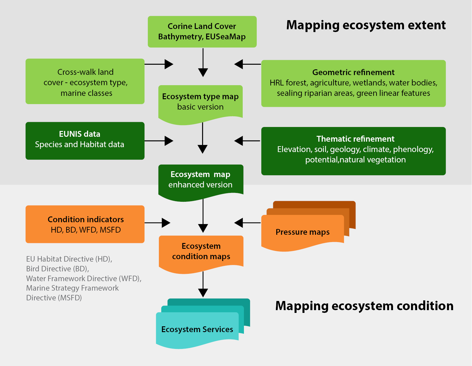
For policy-relevant information, the map should be re-classified using an ecosystem typology which represents the most important types of their human management to make best use of their services, e.g. by agriculture, forestry, fisheries, water management, nature protection or territorial planning. These management lines are also usually implemented in the respective legislations which are important cornerstones in the decision-making process. In case further geometric refinements are required, these can be performed by, for example, integrating more detailed information about rivers and lakes, green linear elements such as hedgerows or detailed maps of urban areas or protected areas.
If needed, such a basic map can be further refined thematically by providing more detailed information about the natural characteristics of the ecosystems and their biodiversity. GIS-based, so-called envelope- or niche-modelling as developed for habitat or climate change impact studies, allows the combination of non-spatially referenced species or habitat information with a set of environmental parameters such as elevation, soil, geology, climate, phenology, potential natural vegetation etc. to delineate the most likely areas of ecosystem presence.
This probability mapping of ecosystem presence depends on the accuracy of the descriptors of its natural boundaries (e.g. alpine meadows or calcareous broadleaf forests) and the availability and quality of the respective data to delineate and map these boundaries. Further enhancement can be performed by attributing statistical information e.g. crop yields or forest inventory data to the respective ecosystem classes.
Mapping ecosystem conditions
Mapping of ecosystem types provides information on the natural conditions. To assess the current capability of ecosystems to provide services for human well-being requires information about their current conditions which are induced by human activities.
For decision support, the most comprehensive and informative approach for the assessment of ecosystem conditions should include direct mapping and assessments in combination with information about the direct and indirect pressures which induce these conditions. This approach provides information on both the current environmental state and expected changes due to constant, increasing or decreasing pressures. Additionally, important information for risk assessments can be derived. Time lags between pressures and changes in ecosystem conditions are often triggered by buffering processes which indicate the resilience of species and ecosystems to the different types of stress factors affecting their condition.
For better understanding of the different processes affecting ecosystem condition and the link to human activities, the DPSIR (Drivers, Pressures, State or Condition, Impact, Response) approach is often used (Figure
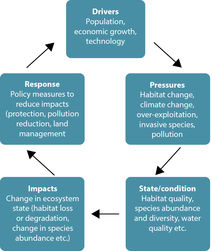
Pressures affect ecosystem conditions either by concentration (e.g. ozone) or by accumulation (e.g. nitrogen and pollution load). The Millennium Ecosystem Assessment 2005 identified five different anthropogenic main pressures affecting ecosystem conditions: habitat change, climate change, invasive species, land management and pollution/nutrient enrichment.
Human pressures are either direct, i.e. mainly from land use, or indirect, i.e. by air pollution or anthropogenic climate change. Important for ecosystem conditions are the strength of the pressure signal, its persistence if cumulative and its change over time. Time-series of observed changes in pressures are, therefore, important to analyse the causal connectivities between pressures and current condition for each ecosystem type and each spatial unit. The trend in pressures also provides a first insight into the expected changes in the near future. Decreasing observed trends may indicate further improvement of ecosystem conditions and vice versa, i.e. important information for decision-making about measures to mitigate and adapt to positive or negative effects.
For the implementation of the EU Biodiversity Strategy to 2020, Member Countries and European institutions perform ecosystem assessments in their territories. The European map is based on a proxy following the scheme as outlined in Figure
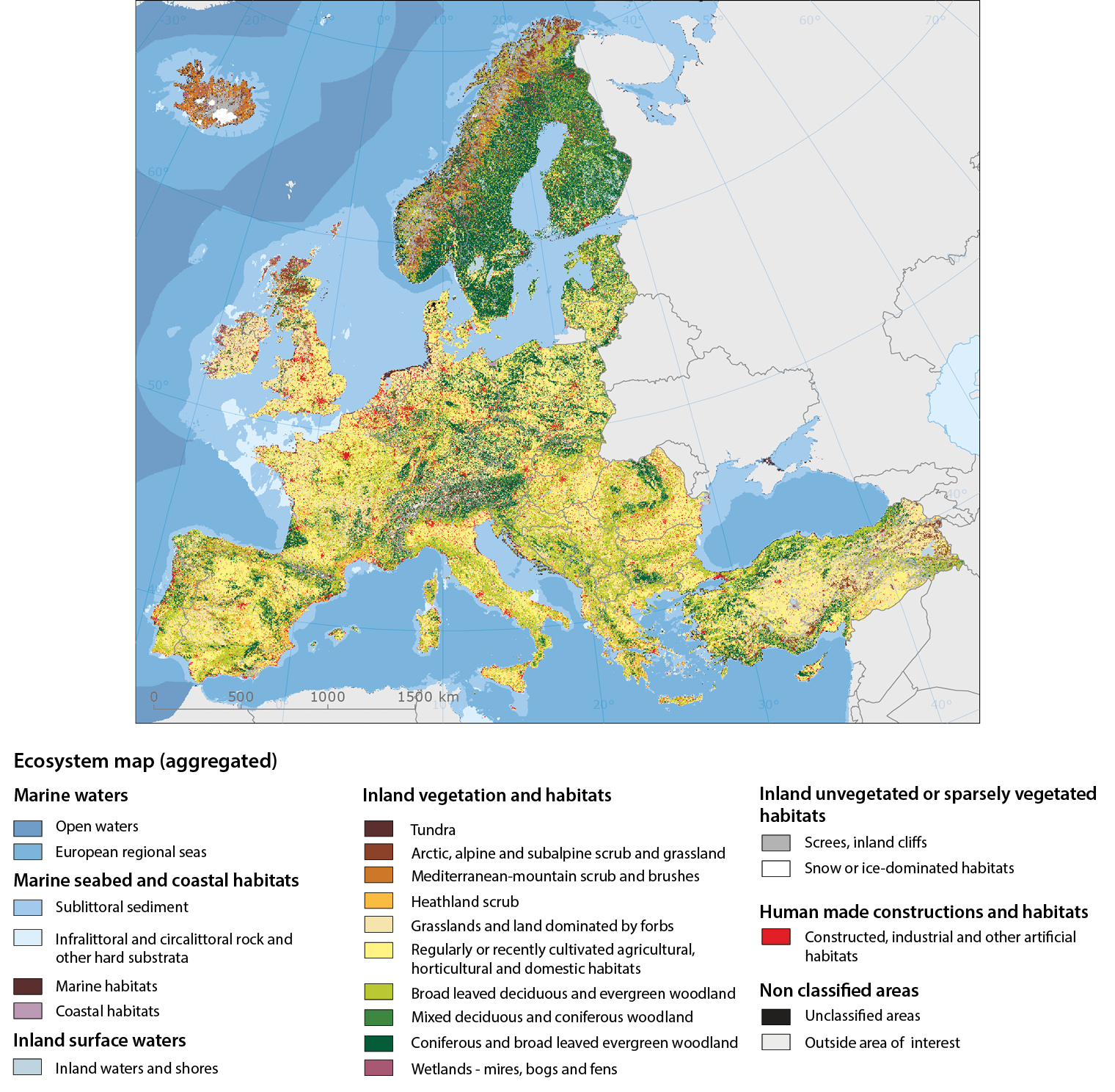
Ecosystem map of Europe Version 2.1 (higher resolution map can be downloaded at: http://www.eea.europa.eu/data-and-maps/data/ecosystem-types-of-europe).
In practice, information on ecosystem conditions is often insufficient for appropriate mapping and assessments. Another problem is the mapping and assessment of the combined effects of pressures on the ecosystem condition. Usually spatially explicit maps of the different pressures and their gradients across the area under investigation can be produced but knowledge about the combined effects on biodiversity and ecosystem structure and function is still insufficient. So in many cases, proxy indicators have to be used to indicate the current ecosystem condition as illustrated in Box 2.
Figure
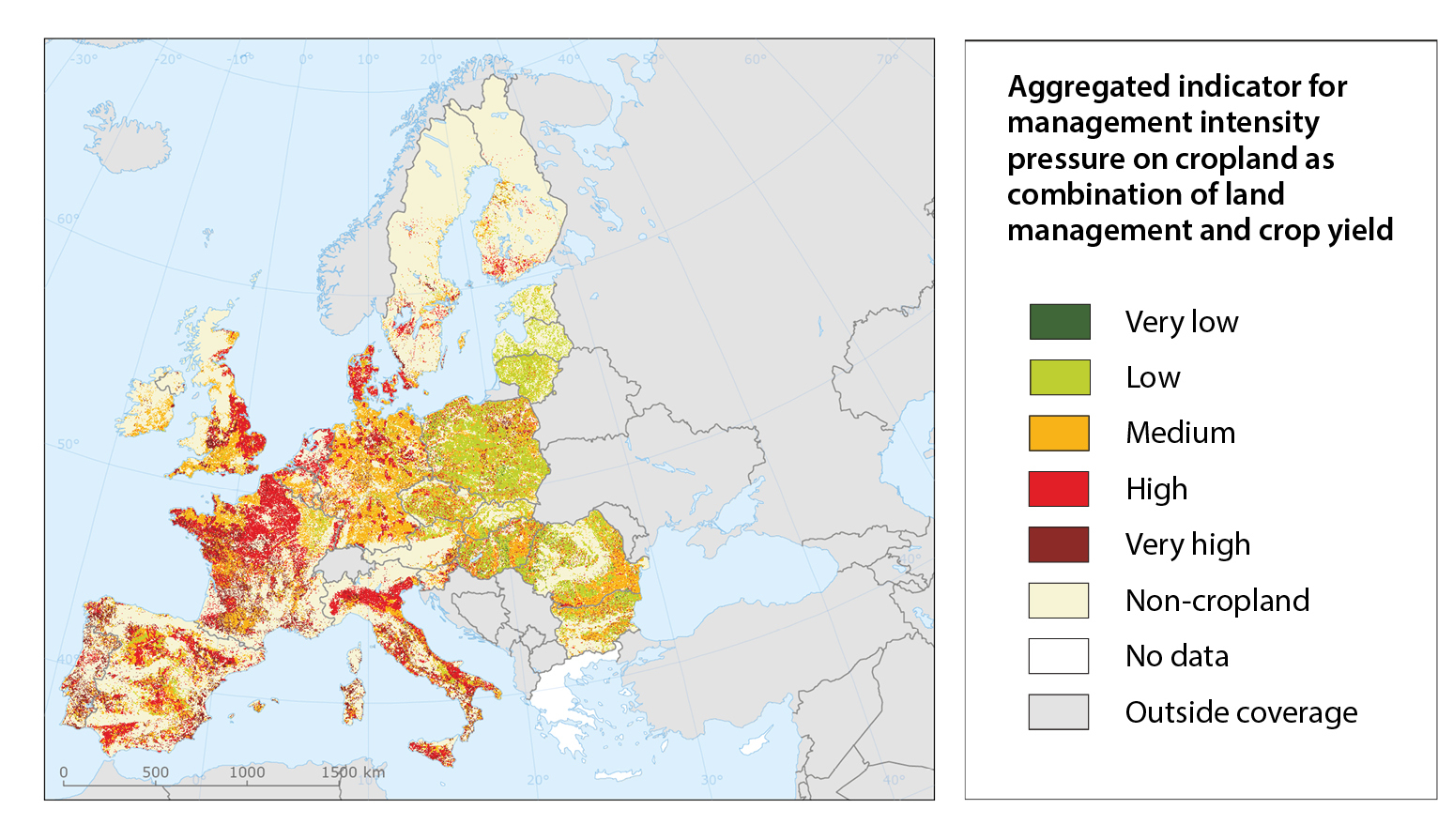
The way forward
Ecosystem type mapping and condition assessments have to be further improved making use of new information and data flows from research, reporting and other sources.
A major issue is the lack of detailed information on how the ecosystem condition affects ecosystem service delivery. The delivery of ecosystem services depends on the biological, physical and chemical processes and the biodiversity involved (Chapters 2.2 and 2.3) but there are few quantitative data to model and assess how these processes and functional traits are affected by pressures such as pollution, management or climate change and their combined effects. Further research is needed to fill these gaps and improve our knowledge about the relationships between pressures - ecosystem conditions, related biodiversity and ecosystem service capacity.
Further reading
- De Groot RS, Alkemade R, Braat L, Hein L, Willemen L (2010) Challenges in integrating the concept of ecosystem services and values in landscape planning, management and decision making. Ecological Complexity 7: 260-272.
- EEA (2016) Mapping and assessing the condition of Europe's ecosystems: progress and challenges. EEA report 03/2016 http://www.eea.europa.eu/publications/mapping-europes-ecosystems accessed 31 May 2016.
- Harrison PA, Berry PM, Simpson G, Haslett JR, Blicharska M, Bucur M, Dunford R, Egoh B, Garcia-Llorente M, Geam N, Geertsema W, Lommelen E, Meiresonne L, Turkelboom F (2014) Linkages between biodiversity attributes and ecosystem services: A systematic review. Ecosystem Services 9: 191-203.
- Maes J, Teller A, Erhard M et al. (2013) Mapping and Assessment of Ecosystems and their Services. An analytical framework for ecosystem assessments under action 5 of the EU biodiversity strategy to 2020. Publications office of the European Union, Luxembourg http://ec.europa.eu/environment/nature/knowledge/ecosystem_assessment/pdf/MAESWorkingPaper2013.pdf accessed 12 December 2015.
- MAES information platform: Mapping and Assessment of Ecosystems and their Services (MAES): http://biodiversity.europa.eu/maes accessed 31 May 2016.
- Millennium Ecosystem Assessment (2005) Ecosystems and human well-being: Synthesis, Millennium Ecosystem Assessment, Island Press, Washington, DC, USA: http://www.maweb.org/en/index.aspx accessed 31 May 2016.
- Potschin M, Haines-Young R, Fish R, Turner RK (Eds.) (2016) Routledge Handbook of Ecosystem Services. Routledge London and New York 629 pp.
3.6. Landscape metrics
Introduction
Landscape metrics have been used to derive indicators in landscape ecology and related disciplines for decades. More than one hundred metrics have been developed for the purpose of describing processes and landscape functions in the form of mathematical terms. After a very enthusiastic time, the focus at present is on meaningful, simpler measures that can be applied in practice. Meanwhile, landscape metrics play a crucial role not only in science, but also in practical issues, such as spatial planning or biodiversity monitoring. Most frequently applied metrics are used to discover biodiversity or landscape fragmentation. Although great advances have already been made, new metrics continue to be developed. Regularly used metrics are further tested and updated regarding their interpretation. This subject is not without controversy. A question which is often raised in research circles is:
Which role can landscape metrics play within the set of indicators for ES mapping and assessment?
The following sections address this question. Regarding the ES cascade model (Chapter 2.3) and following on from it, landscape structures support biodiversity and ecosystem functions that are the basis for the final provision of ecosystem services (ES) to humans. The crucial question is whether landscape metrics applied to land use / land cover maps can provide direct or indirect indications on the provision of ES.
So far, landscape metrics have been applied to indicate cultural ES (e.g. recreation, landscape aesthetics) and regulating ES (e.g. soil erosion, biological pest control). However they are predominantly applied to measure ecological functioning (biodiversity, connectivity, soil quality) and land use processes (land consumption, fragmentation, urban sprawl).
Within this chapter, we review the know-ledge of pattern-related challenges in ES mapping, using the examples of habitat connectivity and scenic attraction. We contribute to a better understanding of the reasons for challenges in mapping structure-dependent ES and we demonstrate some methods for addressing them.
Landscape metrics as method for ES mapping
Landscape metrics are tools which can be used to bridge the methodological gap between landscape structure and ES provision. They take the visible spatial manifestation of land use patterns into account. Composition and configuration of patches (homogeneous units of one property, e.g. land use type) are key features of maps. Hence, landscape metrics and mapping are inherently interrelated. Table 1 provides an overview of selected landscape metrics which are applicable for mapping and assessment of ES.
Examples for suitable landscape metrics indicating biodiversity and ES (provisioning, regulating, cultural; following CICES (2013)), without claim to completeness.
| Structure/landscape metric | Process/function | Mapping target |
| Dimension of Biodiversity | ||
| Shannon's diversity index, Patch density ? | Pattern heterogeneity and variety ? | Landscape diversity |
| Shape index ? | Natural conditions ? | Species diversity |
| Proximity index, Nearest neighbour index ? | Isolation, Habitat connectivity ? | Species diversity |
| Effective mesh size ? | Fragmentation ? | Species diversity |
| Provisioning service | ||
| Total patch area (of arable land) ? | Food and fodder production ? | Food and fodder |
| Total patch area (of forested/arable land) ? | Biomass production ? | Biomass |
| Total patch area of lakes ? | Food (fish) | |
| Regulating service | ||
| No. / length of landscape elements (hedges, tree lines) ? | Soil erosion due to water runoff ? | Mass flow |
| Edge length (of hedges, forests and other ecotones) ? | Habitat provision forpollinators (fringe structures) ? | Pollination |
| Shannon's diversity index / Heterogeneity of agricultural areas ? | Population development ? | Pest control |
| Cultural service | ||
| Total patch area (of water), Edge length of waters ? | Attraction, Complexity ? | Landscape aesthetics |
| Shape index Hemeroby index ? | Complexity and Natural conditions ? | Landscape aesthetics |
| No. of landscape elements ? | Legibility, mystery ? | Landscape aesthetics |
Landscape metrics quantify physical landscape structures which themselves determine processes and functions. Although some landscape structures can be measured and related to the provision of specific ES, direct functional interpretation of single metrics regarding ES remains limited. For the assessment and interpretation of landscape metrics, for example, a normative assessment basis is required which relates the current situation of landscape structure to a reference or target situation of ES provision. However, landscape structure is important information in a more complex evaluation of ES. Landscape metrics have therefore to be considered as meaningful parameters together with others in ES mapping and evaluation. A sound application of landscape metrics is possible considering two dimensions of biodiversity, species and landscape diversity. Many species and species communities rely on specific landscape structures or landscape elements and their interrelations.
Provisioning services strongly depend on the extent of managed land and the land use intensity. However, for quantification of productivity or food provision, further information, for example on soil quality or soil management, is essential to derive a valid estimation on food provision. Regarding regulating services, landscape metrics also comprise the potential to provide supplementary information. Indices like edge length or the number of landscape elements can quantify some preconditions for functions and services. Although modelling and/or measurement of species abundance or mass flows (qualitative data; Chapter 4.1) cannot be replaced by structural indicators, they have to be considered as one important part of the required information.
Strong interrelations between indices of biodiversity and landscape aesthetics can be identified as potential of landscape metrics application in mapping ES. Cultural services such as the potential of landscapes for human recreation are interrelated with structural aspects. However, landscape aesthetics is just one of many spiritual, experiential and educational services. Landscape metrics can therefore serve as a complementary mapping and assessment method for cultural ES.
Application of landscape metrics for ES mapping
Landscape metrics have been applied in several ES mapping and assessment studies. Two examples illustrate how they can be related to ecological integrity, considered as the basis for any ES provision (Box 1) and scenic attraction, as an example for cultural ES (Box 2). In a similar manner, spatial structures strongly determine regulating ES. The regulation of soil erosion, for example, can be estimated using the number and the spatial arrangement of landscape elements, such as hedgerows. These elements reduce slope lengths which is one driving factor for soil erosion. However, suitable landscape metrics, such as the number of patches or edge length, have not been frequently used for assessment and mapping of regulating ES.
One approach, how landscape metrics can contribute to ES mapping and assessment, is illustrated in Figure 1. Six metrics were applied to an administrative planning region (3,434 km?) in middle Saxony, Germany to evaluate ecological integrity as the precondition for biodiversity and the cultural service landscape aesthetics. They were implemented into the land use change simulation software GISCAME as supplementary indicators. In this software, the basic evaluation of ES is based on land use types. An additional landscape structure add-on makes the impact of composition and configuration visible and assessable.
The example focuses on habitat connectivity which is a landscape function related to biodiversity (see Table 1). Using the "moving window" method, which is independent from any administrative or geographical zoning, combined with a cost-distance analysis, local landscape pattern were examined across space and interpreted. The size of the moving window is determined by the action radius of a target species. On the basis of the degree of hemeroby of land use types, near-to-nature areas were identified, as well as core habitat areas and functionally connected areas. The latter were defined as potential habitat areas which are too small and not compact enough to provide habitat core areas. Nevertheless, they are close enough to another core area to be appropriate habitats for species moving through a landscape. Such functionally connected areas were also considered as part of the habitat network. (Semi-)natural areas were considered as isolated and therefore not contributing to the habitat network if they were separated by roads, urban areas and similar land use types acting as barriers.
The map in has been classified according to the functional interpretation of a land use map. It can serve scientists as well as spatial planners to identify i) the share of land which contributes to a habitat network and ii) its spatial distribution. This information allows spatially explicit conclusions on priority areas for enhancement of the connectivity and on the overall state of habitat connectivity as one influencing factor of biodiversity.
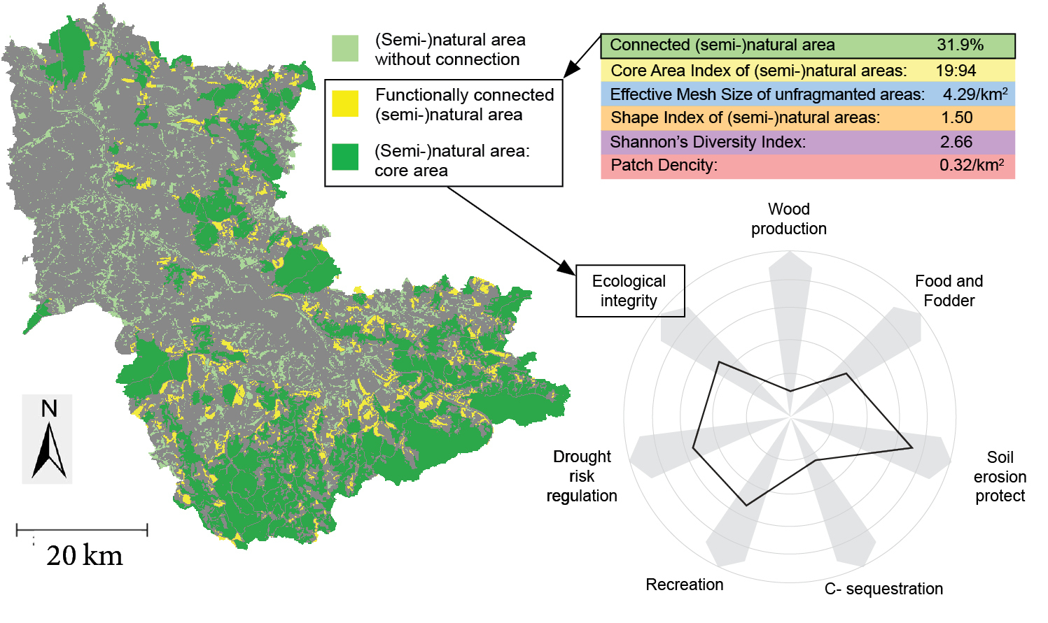
Based on the natural amenities and features, a model for assessing the scenic attraction of landscapes is presented. It is a suitability analysis of an area for nature-based recreation, assuming that certain features of the landscape have a positive or negative impact on the attraction of the landscape and recreation. In this model, landscape metrics are used for several parameters. The relief diversity, the proportion of open space, the hemeroby Index, the density of forest-dominated ecotones, the density of water edges (without coasts), the coastlines and the proportion of unfragmented open space greater 50 km? were selected.
The relief diversity (ratio 3D / 2D) reflects not only the maximum height difference (relief energy), but also the cumulative differences in altitude. A low proportion of open space indicates urban or densely built-up areas which can decrease the natural attraction of the landscape by the strong influence of technical artefacts. In congruence with the hemeroby index, the natural condition is an important factor for the attraction of landscapes. With the density of ecotones dominated by trees and shrubs and the density of water edges, landscape diversity and structure are taken into account. This parameter characterises mainly the variety and edge effects. Since the coasts play a very important role in terms of attraction and recreation, they are represented by their own parameters - coastlines. Finally, the disturbing effect of fragmentation by the transport network is considered with the parameter 'proportion of unfragmented open spaces greater than 50 km?'.
All data used were based on the official land use data of the state and federal German survey authorities (ATKIS Basis DLM or land cover model LBM-DE) in vector format collected in 2010. The indicator of the scenic attraction was calculated based on a 5-km grid (standardised according to EU INSPIRE directive).
To determine the five classes of scenic attraction, the standard deviation from the nationwide average was used. The reason behind this approach is mainly to use no fixed scale, but starting from the average values of the scenic attraction, to be able to make statements as to whether an area is rather less, or rather more scenically attractive. Landscapes which are significantly affected by anthropogenic impacts and thus often are particularly fragmented, intensively farmed or settled, can be found in the class "less attractive". Average attractive landscapes already meet recreational functions in a regional context, while very or particularly attractive landscapes represent targets for nature-related tourism and are mostly well-known nationwide.
Monitoring the development of scenic attraction using this aggregated indicator would provide decision-makers with indications as to where the scenic attraction is particularly reduced or has improved. The information derived from the aggregated, landscape metrics-based indicator reveals that individual changes affect the landscape values in their sum. Furthermore, spatial information on the scenic attraction can be used to avoid encroachments in scenic highly attractive areas and thus to achieve better management.
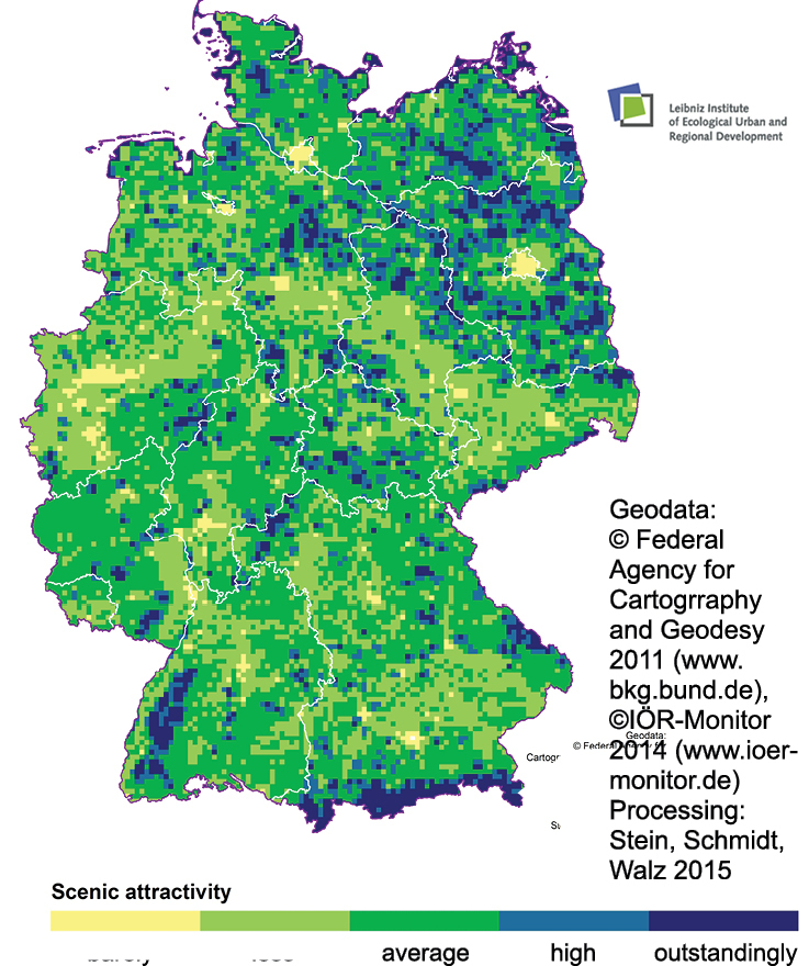
Furthermore, small-scale landscape elements such as ecotones at forest borders, single-trees, hedgerows including field margins are important for the regulating of ES pollination.
Conclusions
Landscape metrics and ES mapping are inherently related topics since landscape metrics quantify spatial characteristics of landscape patterns. Therefore, we recommend the application of landscape metrics in the context of ES mapping and also ES assessment. These indices have the power to support the identification and monitoring of spatial characteristics of landscapes which have implications on the perfor mance of biodiversity and several ES.
Some dimensions of biodiversity and cultural ES can be comprehensively indicated by landscape metrics.
The validity and verifiability of landscape metrics, however, is limited. They quantify and illustrate processes and/or functions, which can serve as surrogates for specific ES. Due to such indirect links to ES, landscape metrics should only be used as supplementary indicators for ES assessments. In the case of landscape aesthetics and recreation, they can be more directly linked to the ES provision. However, landscape metrics describe structural aspects of ES (which are important and should not be forgotten), but usually additional information (e.g. data on quality of land use) is necessary. Still, they have a great significance in terms of mapping.
The spatial interpretation of land use maps with the help of landscape metrics serves as a valuable method for communicating ES-related issues. With regard to the current application for ES mapping and assessment in science and practice, we foresee a large capacity for future application of landscape metrics, especially in practice. The benefit of using landscape metrics for ES mapping is currently below its estimated potential.
Further reading
- Burkhard B, Kandziora M, Hou Y, Muller F (2014) Ecosystem Service Potentials, Flows and Demands - Concepts for Spatial Localisation, Indication and Quantification. Landscape Online 34: 1-32.
- Botequilha Leitao A, Ahern J, McGarigal K (2006) Measuring Landscapes. A Planner's Handbook. Island Press; 2nd edition.
- Frank S, Furst C, Koschke L, Makeschin F (2012) A contribution towards a transfer of the ecosystem service concept to landscape planning using landscape metrics. Ecological Indicators 21: 30-38.
- Haines-Young R, Potschin M (2013) Common International Classification of EcosystemServices (CICES), version 4.3. Report to the European Environment Agency EEA/BSS/07/007 (download: www.cices.eu).
- McGarigal (2015) FRAGSTATS HELP. V. 4.2, 21 April 2015, available online: http://books.umass.edu/landeco/research/fragstats/documents/fragstats.help.4.2.pdf
- Walz U, Stein C (2014) Indicators of hemeroby for the monitoring of landscapes in Germany. Journal for Nature Conservation 22(3): 279-289.
- Walz U (2015) Indicators to monitor the structural diversity of landscapes. Ecological Modelling 295: 88-106.
3.7. Specific challenges of mapping ecosystem services
Ecosystems are spatially explicit and so too are their conditions and their capacity to provide ecosystem services (ES). The different biomes and ecosystems that cover the earth's surface deliver various ES bundles at different quantities and qualities. These services are often consumed or used at other places. Mapping ES thus makes good sense, in particular to quantify and sum stocks and flows (Chapter 5.1) of services at different spatial scales (Chapter 5.7).
Furthermore, maps are very powerful tools for communicating and organising data. It is little wonder that geography is a major subject at school. Most people are familiar with maps to navigate or to find places for holidays or recreation. Maps are used to present data and compare the performance of countries and regions across the world for virtually all possible indicators. Many of us have still paper maps in our cars or digital maps on our cell phones, as well as the popular Google Maps which are an essential tool and benefit to our lives.
It follows that there is a strong basis in our society for maps and mapping and thus for mapping ecosystem services as well. In particular, there is a demand from policy-makers to map ES (see Chapter 7.1) and to build natural capital accounts which should be based on the reliable geo-referenced data of ecosystems.
Despite the popularity of maps, they are pitfalls as well. Some claim that "maps have an air of authority". Which means that maps and their content are often taken for granted. Yet, ES mapping is challenging for a number of reasons. These are listed here while referring to the next chapters which present and discuss solutions for addressing these challenges.
An often heard challenge is that not all ES can be mapped. Review articles typically found that regulating and provisioning ES are most frequently mapped but cultural ES less so. As for regulating ES, most efforts have gone to mapping climate regulation while for provisioning ES, the focus is on food, water and timber. Evidently, these mapping studies have largely profited from knowledge stemming from environmental sciences and agricultural and forestry research. However, substantial progress in mapping ES has been made in the recent decade (see chapters 5.5.1, 5.5.2 and 5.5.3) and solutions have been found to map services which were previously thought impossible to map (see chapter 6.2). Particular advancements have been realised to map certain cultural ES or to map regulating ES which involve service providing areas (Chapter 5.2) that operate at very small spatial scales (such as pollination or biological control).
A specific challenge is related to the trans-disciplinary nature of ecosystem services. ES research has become a major academic field, drawing on various academic disciplines, perspectives and research approaches. The multifaceted ES concept includes, in addition, a normative component. This exposes ES maps (and the researchers who created them) to the general critique of not being sufficiently inclusive and to the specific critique from disciplinary specialists of oversimplifying detailed ecological processes that are underpinning ES. To both challenges the ES mapping community has responded well. Chapter 5.6 demonstrates how different views expressed by different stakeholders and researchers can be accommodated in the ES framework. Mapping ES nowadays is not restricted to natural sciences but includes social and economic sciences as well. Furthermore, recent studies promote the adoption of a tiered mapping approach which allows increasing levels of spatial and ecological details to be incorporated in mapping studies (chapter 5.6.1).
Besides these thematic challenges, there are significant technical challenges to map ES.
A question which often arises relates to what ES maps should express: ES potentials, flows or demand (Chapter 5.1)? ES are realised when humans benefit from them. At this point, supply meets demand and ES "flow" from where they are generated to where they are received (Chapter 5.2). These flows are dynamic over time and therefore difficult to capture on maps; stocks exhibit less dynamics and are therefore easier to map. A typical example is climate regulation; this service is often mapped by the carbon stock in soil or above-ground vegetation assuming that the stock is related to the capacity to provide a flow of service. Carbon capture as such is less mapped. The notion of stocks and flows is crucial for accounting purposes. The size of the stock is not necessarily related to the magnitude of ES flows, so this challenge needs to be addressed when ES maps are applied in decision-making contexts.
The selection of an appropriate spatial scale and an appropriate mapping unit is another important issue and remains a challenge for ES mapping studies (Chapter 5.7). Ecological processes occur at different spatial and temporal scales. Pollination by insects is, for example, a very local ES which takes place in a specific period of the year when temperature allows bees and other pollinators to be active. Groundwater recharge, in contrast, is a large-scale process which usually is measured in decades. ES related to water, climate and atmosphere demonstrate entirely different behaviour from services related to soil. They require different quantification approaches and are measured for different spatial units. This results in maps which vary across scale and spatial unit. Bringing them together in a series of consistent and harmonised ES maps for spatial planning and policy support requires application of spatial operations (such as upscaling, downscaling, spatial statistics) which, in turn, may introduce uncertainties (Chapter 6). Using scalable indicators (e.g. indicators which can be measured at different spatial scales such as the density of trees) could overcome errors that arise when local data are upscaled or when global data are downscaled. But such indicators are not always available. In particular for water, air and soil, related ES measurements are mostly local and not scalable to larger spatial scales.
ES mapping could thus be substantially advanced by a more systematic development of cross-case comparisons and methods. Several chapters of this book touch on these challenges related to spatial scale and provide solutions for dealing with uncertainties arising from spatial data handling (different sections under 5.7). As more efforts and research are focused on these areas, it seems likely that datasets generated at different spatial and temporal scales and, using different types of data, will complement one another to provide a coherent message regarding the health of global ecosystems, biodiversity and the benefits they confer upon society.
The different thematic and methodological challenges are sources of uncertainties that should be considered when using ES maps. ES map-makers should try to detect sources of uncertainty and give guidance on how to deal with them (Chapter 6.3). Of equal importance is transparency. The map-maker should be clear about how the maps are generated. A helpful tool is provided by the Blueprint for mapping and modelling ES (see further reading and Chapter 7.9). The primary purpose of this blueprint is to provide a template and checklist of information needed for those carrying out an ES modelling and mapping study. A second purpose is to reduce uncertainties associated with quantifying and mapping of ES and thereby help to close the gap between theory and practice.
Further reading
- Abson DJ, von Wehrden H, Baumgartner S, Fischer J, Hanspach J, Hardtle W, Heinrichs H, Klein AM, Lang DJ, Martens P, Walmsley D (2014) Ecosystem services as a boundary object for sustainability. Ecological Economics 103: 29-37.
- Crossman ND, Burkhard B Nedkov S, Willemen L, Petz K, Palomo I, Drakou EG, Martin-Lopez B, McPhearson T, Boyanova K, Alkemade R, Egoh B, Dunbar MB, Maes J (2013) A blueprint for mapping and modelling ecosystem services. Ecosystem Services 4: 4-14.
- Dick J, Maes J, Smith RI, Paracchini ML, Zulian G (2014) Cross-scale analysis of ecosystem services identified and assessed at local and European level. Ecological Indicators 38: 20-30.
- Hauck J, Gorg C, Varjopuro R, Ratamaki O, Maes J, Wittmer H, Jax K (2013) Maps have an air of authority: Potential benefits and challenges of ecosystem service maps at different levels of decision making. Ecosystem Services 4: 25-32.
- Martnez-Harms MJ, Balvanera P (2012) Methods for mapping ecosystem service supply: A review. International Journal of Biodiversity Science, Ecosystems Services and Management 8: 17-25.
Chapter 4. Ecosystem services quantification
4.1. Biophysical quantification
Introduction
Ecosystem services (ES) arise when ecological structures and ecological processes directly or indirectly contribute to human well-being and meet a certain demand from people. This flow of ES from ecosystems to society is well represented by the ES cascade concept (see Chapter 2.3). Ecosystems provide the necessary structure and processes that underpin ecosystem functions which are defined as the capacity or potential to deliver services. ES are derived from ecosystem functions and represent the realised flow of services in relation to the benefits and values of people. This model is useful for quantifying ES. Consider the following example: wetlands (an ecosystem or a structure) provide habitat for bacteria which break down excess nitrogen (denitrification, a process). This results in the removal of nitrogen from the water (a service) resulting in better water quality (a benefit). People can value increased water quality in multiple ways (e.g., by expressing their willingness to pay for clean water). Each of these different steps can be quantified using biophysical, economic or social valuation methods.
This chapter focuses on biophysical quantification which is the measurement of ES in biophysical units. Biophysical units are used to express, for example, quantities of water abstracted from a lake, area of forest or stocks of carbon in the soil. Looking at the ES cascade, it seems evident that biophysical quantification focuses, in particular, on the measurement of ecosystem structures, processes, functions and service flows (also known as the left side or the supply side of the cascade). Benefits and values (also known as the right side or demand side of the cascade) are more often measured using social (see Chapter 4.2) or economic units (see Chapter 4.3). Nonetheless, benefits and values can sometimes be expressed in biophysical units as well. Consider again the above example of water purification in wetlands. The benefit from this ecosystem service is clean water and this can be expressed as the concentration of pollutant substances.
To quantify ES along the different components of the ES cascade, we need to address two questions: what do we measure and how do we measure (Figure
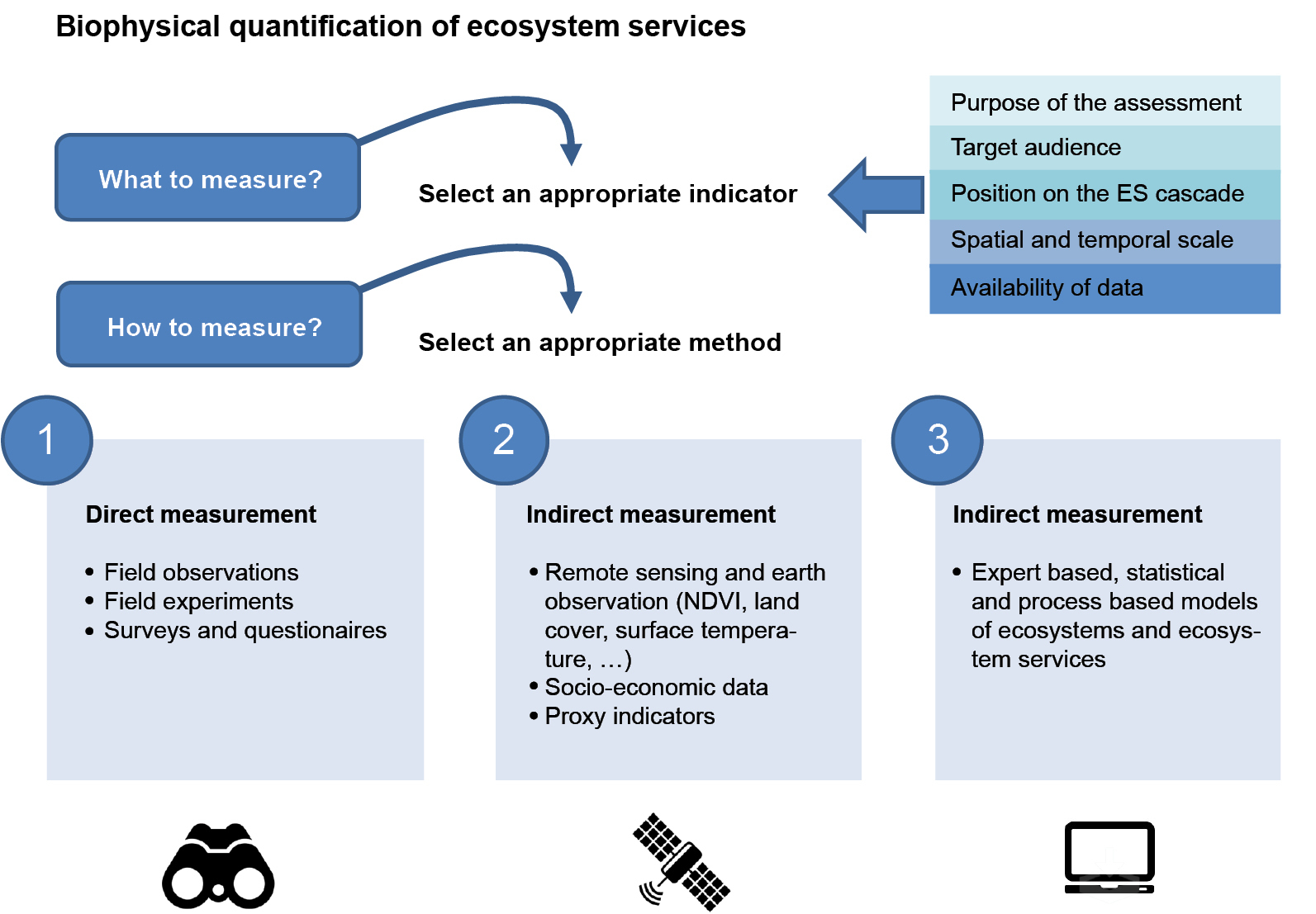
The first question is addressed in the scientific literature by developing and proposing indicators. Ecosystem service indicators are used to monitor the state or trends of ecosystems and ecosystem service delivery within a determined time interval. In recent years a substantial indicator base has been developed world wide to assess or measure ES.
Once an indicator is proposed or selected for inclusion in an ecosystem assessment, the second question becomes important: how can we measure the service or the indicator in biophysical terms or units? Which methods or procedures should be applied to come to an reasonable estimate of the quantity of service provided?
What to measure: Ecosystem service indicators
ES indicators are information that efficiently communicates the characteristics and trends of ES, making it possible for policy-makers to understand the condition, trends and rate of change in ES.
Different indicators can be used to measure or indicate a single ecosystem service. The choice for an indicator depends on many factors including the purpose, the audience, its position on the ES cascade, the spatial and temporal scale considered and the availability of data.
Purpose and target audience are important criteria for selecting or designing indicators for ES. It makes a difference if indicators are used to inform policy makers, journalists, conservation and land managers, scientists or students. Not everybody has an equal understanding of the flow of ES which is indeed a relatively complex concept. Therefore, indicators are sometimes expressed in relative terms by setting a reference value equal to, for instance, 100 and by calculating other values relative to this reference. This facilitates interpretation for some user groups. Of equal importance is the purpose of an indicator. Why is it used? Many ES indicators are proposed to report the state and trends of ES under different biodiversity policies from global to local scale. But such indicators are not necessarily useful for application by spatial planners or for scientific support to river basin management. Consider pollination, a regulating ecosystem service. A scientist could be interested in the diversity and density of different bee and bumblebee populations; a farmer may wish to know how far he can rely on wild pollination to help pollinate his fruit trees; a biodiversity policy officer may need to know if, at national scale, pollination services are declining or increasing. Clearly, these stakeholders have different information requests which require different indicators with different biophysical units although pollination is the common denominator.
The above example also illustrates the importance of spatial and temporal scales. The issue of scale is frequently presented in all textbooks on ecology as biodiversity and the ecological processes it supports (and thus also the delivery of ES) are heavily dependent on time and space. Processes are influenced by different time cycles (day-night, seasons) and take place at different rates (see also Chapter 5.3). The self-purifying capacity of water is, for instance, highly dependent on the velocity at which water flows. Water purification services, for example, which can be measured by the amount of pollutant removed, differ between fast running streams and stagnant lakes with the latter ecosystems having, in general, a higher capacity (more time) to remove nitrogen but a lower capacity to clean organic pollution. Also spatial scale matters. Bees and bumblebees deliver their pollination services within a distance of a few hundred metres whereas the storage of carbon in trees operates at almost global scale. Indicators and, in particular, their units of measurement have to consider the scale at which ES are relevant. Sometimes indicators are designed to be scale independent. This means they can be upscaled or downscaled, a very useful technique for mapping.
An important question often raised in literature on ES is: should indicators measure the stock and the flow? A service flow refers to the actual use of the actual benefits people receive from ecosystems. A stock refers to the capacity of ecosystems to deliver those benefits. Flows are always expressed per unit of time. Timber production serves as a good example to illustrate the difference between an indicator which measures the stock and an indicator which measures the flow. Timber production is often measured by quantifying the harvest (how much timber is cut, usually expressed in a volume of wood per unit area and per unit of time, for example, m3/ha/year). Sometimes timber production can also be indicated by the available timber stock which can be harvested. This difference is subtle for the case of timber. If the stock is harvested, stock becomes flow. However, for other services, the difference between stock and flow is important because indicators for stock and flow cannot always be expressed in the same units. Wetlands have a certain capacity to clean water but it is not always straightforward to express this capacity in terms of pollutant removal (e.g., amount of nitrogen removed or immobilised in the sediment in kg/ha/year). Often the size of the wetland (in ha) is used as proxy to indicate this capacity. The rationale is that larger wetlands have more capacity to purify water than smaller wetlands. In this context, the concept of ecosystem condition is important as well (see Chapter 3.5). Not only the quantity (spatial extent) of an ecosystem is important to assess the physical values of ES capacity, ecosystem quality or ecosystem condition is also an important determinant of ecosystem delivery. Changes in ecosystems through degradation can thus alter the flows of ES and should thus be measured as well by indicators.
A final remark on indicators relates to composite indicators or indices which aggregate different sorts of information into a single number. Usually such indicators are made for specific purposes or to inform on particular challenges with a single value. In a similar context for ES, such indicators exist but usually they are composed of normalised versions of indicators for single services which are summed or aggregated. They cannot be quantified directly but depend on separate quantification of their individual components.
This chapter does not provide a list with indicators for ES for the simple reason that there are hundreds of indicators available. Many countries and regions have developed ES indicator sets; the setting of global or regional biodiversity targets has also spurred the development of indicators. Furthermore, the application of the ES concept for planning, natural resources management and conservation has created additional indicators. Therefore we list in Table
Examples of sources, websites and key publications for ecosystem service indicators.
| Scale | Location | Publication |
| Global | Measuring Nature's Benefits: A Preliminary Roadmap for Improving Ecosystem Service Indicators (http://pdf.wri.org/measuring_natures_benefits.pdf) http://www.bipindicators.net/ (report ISBN 92-9225-376-X) Measuring ecosystem services: Guidance on developing ecosystem service indicators (ISBN: 978-92-807-4919-5) http://es-partnership.org/community/workings-groups/thematic-working-groups/twg-3-es-indicators/; A Global System for Monitoring Ecosystem Service Change (doi: 10.1525/bio.2012.62.11.7) | |
| Sub-global | European Union | website: http://biodiversity.europa.eu/maes/mapping-ecosystems; article: doi: 10.1016/j.ecoser.2015.10.023 |
| National | Finland | website: http://www.biodiversity.fi/ecosystemservices/home; article: doi: 10.1016/j.ecolind.2015.03.041 |
| Canada | Website: https://www.ec.gc.ca/indicateurs-indicators/ | |
| Switzerland | Website: http://www.bafu.admin.ch/publikationen/publikation/01587/index.html?lang=en | |
| Germany | article: Towards a national set of ecosystem service indicators: Insights from Germany (doi: 10.1016/j.ecolind.2015.08.050) | |
| Spain | Website: http://www.ecomilenio.es/informe-de-resultados-eme/1760; Article: doi: 10.1371/journal.pone.0073249 |
In summary, ES indicators express what to measure when quantifying ES in a biophysical manner. Good ES indicators come with information on their place on the ES cascade, on the available data, on the targeted audience and the objective and on whether they assess a stock or a flow.
How to measure
Indicators must be measured but how is this done for ES? Some of the above given examples already provide the answer. The number of bees on a farmland, the timber harvest from a forest or the denitrification in a wetland can all be monitored or measured with different methods or devices. Yet measuring stocks or flows of ES is less evident than it seems. Here we present three approaches which can be considered to quantify biophysical stocks and flows of ES: direct measurements, indirect measurement and (numerical) modelling.
Direct measurements of ecosystem services
Direct measurements of an ecosystem service indicator is the actual measurement of a state, a quantity or a process from observations, monitoring, surveys or questionnaires which cover the entire study area in a representative manner. Direct measurements of ES deliver a biophysical value of ES in physical units which correspond to the units of the indicator. Direct measurements quantify or measure a stock or a flow value. Direct measurements are also referred to as primary data.
Examples of direct measurements of ES (see also Table
Examples of different methods to measure ecosystem service indicators
| Ecosystem services | What to measure | How to measure (method) | ||
|---|---|---|---|---|
| (CICES class) | Indicator | Direct | Indirect | Model |
| Cultivated crops | Crop yield (tonne/ha/year) | Crop statistics (obtained through official reporting) | Remote sensing of crop biomass using NDVI and aerial photo analysis for long temporal changes Coupling structural observations with remote sensing information | Crop production models |
| Reared animals and their outputs | Livestock (heads/ha) | Livestock statistics (head counts obtained by reporting) | ||
| Wild plants, algae and their outputs | Wild berry yield (tonne/ha/year) | Field observations and surveys of people harvesting wild fruits | Species distribution models; ecological production model | |
| Animals from in-situ aquaculture | Fish yield (tonne/ha/year) | Aquaculture statistics (obtained through official reporting) | Fish production models | |
| Water (Nutrition) | Water abstracted (m3/year) | Water statistics (obtained through official reporting) | Remote sensing of water bodies and soil moisture | Water balance models |
| Biomass (Materials) | Timber growing stock (m3/ha) and timber harvest (m3/ha/year) | Forest stand measurements and forest statistics | Remote sensing of forest biomass using NDVI | Timber production models |
| (Mediation of waste, toxics and other nuisances) | Area occupied by riparian forests (ha) | Site observations | Earth observation land cover data | |
| Nitrogen and Sulphur removal in the atmosphere or in water bodies (kg/ha/year) | Measurement of deposition of NO2 and SO2; field measurement of denitrification in water bodies | Remote sensing of canopy structure (leaf area index) | Transport and fate models for N and S | |
| Mass stabilisation and control of erosion rates | Soil erosion risk (tonne/ha/year) | Field measurements of soil erosion | Soil erosion models (RUSLE) | |
| Flood protection | Area of floodplain and wetlands (ha) | Site observations | Elevation models and data; aerial photo analysis; remote sensing of land cover | Modelling water transport |
| Pollination and seed dispersal | Pollination potential; number and abundance of pollinator species (number/m2) | Field sampling of pollinator species; counts of bee hives | Species distribution models; ecological modelling of habitat suitability | |
| Decomposition and fixing processes | Area of nitrogen fixing crops (ha) | Field surveys; crop statistics (obtained through official reporting) | Crop production models | |
| Global climate regulation by reduction of greenhouse gas concentrations | Carbon storage (in soil or aboveground biomass) (tonne/ha); carbon sequestration (tonne/ha/year) | On-site measurements of carbon stock and carbon fluxes | Remote sensing of vegetation | Carbon cycle models |
| Physical and experiential interactions | Visitor statistics (number/year) | Visitor data and questionnaires of visitors | Monitoring parking lots, mapping trails or camping sites | Modelling potential use of nature reserves by people |
These examples of direct measurement share a number of characteristics. They are time and resource consuming and thus costly, mostly suitable for carrying out at site level or local scale and they measure tangible flows of ES, in particular for provisioning ES. Direct measurements are also feasible in case of a clearly defined service providing species (or areas) such as pollination, bird watching or biological control.
As many of these indicators are effectively measured for other reasons, it is not always needed to set up expensive measurement schemes. Most provisioning ES including crops, fish, timber and water are recorded by national and regional governments. Furthermore, certain species groups and taxa are monitored to assess trends in biodiversity.
TESSA (http://tessa.tools/) is a toolkit for rapid assessment of ES at site level which provides many procedures and suggestions for on-site measurement of ES.
Direct measurements and the use of primary data are the most accurate way to quantify ES but they become impractical and expensive beyond the site level or they are simply not available for all ES.
Therefore the next step to consider for biophysical quantification is indirect measurements.
Indirect measurements of ES
Indirect measurements of ES deliver a biophysical value in physical units but this value needs further interpretation, certain assumptions or data processing, or it needs to be combined in a model with other sources of environmental information before it can be used to measure an ecosystem service. Indirect measurements of ES deliver a biophysical value of ES in physical units which are different from the units of the selected indicator.
In many cases, variables that are collected through remote sensing qualify as indirect measurement. Examples for terrestrial ecosystems are land surface temperature, NDVI (Normalised Difference Vegetation Index), land cover, water layers, leaf area index and primary production. Examples for marine ecosystems include sea surface temperature, chlorophyll A concentration and suspended solids. Many of these data products do not measure stocks or flows of ES but they are highly useful to quantify global climate regulation as well as all those ES which depend directly on the vegetation biomass of ecosystems to regulate or mediate the environment. Soil protection and water regulation, for example, are strongly driven by the presence of vegetation which can be inferred from earth observation datasets. Local climate regulation can be inferred from spatially and temporally explicit patterns of surface temperature. Air filtration by trees and forest is directly related to the canopy structure which, in turn, can be measured by the leaf area index. In addition, micro-climate regulation in cities (temperature reduction during heat waves through evapotranspiration and provision of shade) can be approximated by measuring the total surface area of urban forest.
A specific role is reserved for land cover and land use data which are used for both direct and indirect quantification of ES. Detailed and accurate information on the extent of ecosystems or of ecosystem service providing units, constitute an essential data basis for all ecosystem assessments. Importantly, land data can also be used to quantify demand for ES.
Not all indirect measurements are provided by earth observation. The density of trails and camping sites may provide an indirect estimate of recreation and tourism (Table
Indirect measurements, in particular earth observation, offer substantial advantages. They provide consistent sources of information often with global coverage and they are regularly updated which makes them suitable for natural capital accounting and monitoring trends.
Modelling as alternative to quantify ES
ES modelling can be used to quantify ES if no direct or indirect measurements are available. This is virtually always the case in any ecosystem assessment. With ES modelling, we understand the simulation of supply, use and demand of ES based on ecological and socio-economic input data or knowledge. Models can vary from simple expert based scoring systems to complex ecological models which simulate the planetary cycles of carbon, nitrogen and water. More details are also available in Chapter 4.4
In the context of biophysical quantification, models can be used for spatial and temporal gap filling of direct and indirect measurements, extrapolation of direct and indirect measurements, modelling ES for which there are no measurements available or for scenario analysis.
For regulating services, modelling is sometimes the only option in order to quantify actual ecosystem service flows. This is particularly evident when ecosystems are regulating or mediating stocks and flows of soil, carbon, nitrogen, water or pollutants. Consider soil protection - also termed as erosion regulation or erosion control - which is the role ecosystems and vegetation plays in retaining soil or avoiding soil being eroded as a result of wind or run-off water. Soil erosion can be measured directly on sites which are prone to erosion, usually cropland on slopes. However, estimating the quantity of soil that is not eroded due to the protective cover of vegetation cannot be measured. It can however be modelled by comparing the amount of soil erosion with a model which simulates the presence of vegetation with a model where the protective vegetation cover is deliberately set to zero or to parameters which correspond to parameters for cropland or bare soil. The difference between these two models results in an estimate of avoided soil erosion and can represent the realised service flow. A similar rationale applies to water purification, air quality regulation or other services which exert control on the fate and transport of abiotic and organic material.
Implementing biophysical methods for decision-making
Ecosystem service assessments have increasingly been used to support environmental management policies, mainly based on biophysical and economic indicators. Therefore ES assessments have to integrate data and information on biophysical ecosystem components, including biodiversity, with socio-economic system components and the societal and policy contexts in which they are embedded.
Quantification of ES using biophysical methods have been used for a number of perspectives and for a variety of purposes, including landscape management, natural capital accounting, awareness raising, priority setting of projects or policies and policy instrument design. However, transferring the outcomes of the biophysical assessments to policy is not straightforward and some additional work is required to ensure a minimum degree of consistency and avoid over-simplistic conclusions.
Different methods are relevant at different policy levels (ranging from international, EU, national, regional and local scales). Existing literature frequently acknowledges that, in these cases, the interrelationship between different scales must be taken into consideration, which can pose significant challenges. Broad framings for these methods include the work done globally of the Inter-governmental Platform on Biodiversity and Ecosystem Services (IPBES) and the Mapping and Assessment of Ecosystems and their Services (MAES) in the context of the EU Biodiversity Strategy. The initial methodological work on biophysical methods will be the basis for the assessment of the economic value of ES and promote the integration of these values into accounting and reporting systems.
Conclusions
"You can't manage what you don't measure". This well-known expression is also valid for ES which is, in essence, a concept to guide and support the management of natural resources, ecosystems and socio-ecological systems. ES represent the flows of material, energy and information from ecosystems to society. Accurate measurement of these flows as well as the extent and the condition of ecosystems which support these flows is therefore key to base decisions, to monitor progress to biodiversity targets and to create a sound knowledge base for natural capital.
Further reading
- Boerema A, Rebelo AJ, Bodi MB, Esler KJ, Meire P (2016) Are ecosystem services adequately quantified? Journal of Applied Ecology. DOI: 10.1111/1365-2664.12696.
- De Araujo Barbosa CC, Atkinson PM, Dearing JA (2015) Remote sensing of ecosystem services: a synthetic review. Ecological Indicators 52: 430-443.
- Kareiva P, Tallis H, Ricketts TH, Daily GC, Polasky S (2011) Natural Capital: Theory and Practice of Mapping Ecosystem Services. Oxford University Press, Oxford.
- Mononen L, Auvinen AP, Ahokumpu AL, Ronka M, Aarras N, Tolvanen H, Kamppinen M, Viirret E, Kumpula T, Vihervaara P (2016) National ecosystem service indicators: Measures of social-ecological sustainability. Ecological Indicators 61: 27-37.
- Peh KS-H et al. (2013) TESSA: A toolkit for rapid assessment of ecosystem services at sites of biodiversity conservation importance. Ecosystem Services 5: e51-e57.
- Pettorelli N, Owen HJF, Duncan C (2016) How do we want satellite remote sensing to support biodiversity conservation globally? Methods in Ecology and Evolution 7: 656-665.
4.2. Socio-cultural valuation approaches
Introduction
Any evaluation of ES requires an integrated analysis, taking into account the supply and demand of ES and their biophysical, socio-cultural and economic value dimensions (see Chapters 4.1, 4.2 and 4.3, respectively). Recent literature has acknowledged that many of the contributions on ES valuation still use the term 'value' exclusively in a monetary sense, ignoring the broader contributions of ecosystems and biodiversity to society in terms of cultural, therapeutic, artistic, inspirational, educational, spiritual or aesthetic values.
To fill this scientific gap, literature on socio-cultural valuation approaches has grown in the last ten years, mostly related to cultural ES (Figure

Trends in the scientific literature exploring socio-cultural valuation approaches for cultural ES. Note: this illustration is not representing the total number of published papers on cultural services valuation, but the timeline of publications of the most relevant papers which focus on six cultural ES: non-extractive recreation and tourism (e.g. outdoor recreation, ecotourism), (2) extractive recreation and tourism (e.g. sport fishing, recreational hunting), (3) local ecological knowledge, (4) scientific knowledge and environmental education, (5) spiritual interactions with nature and (6) aesthetic experience.
Despite the increase in the number of publications, socio-cultural valuation approaches have not yet formalised a common methodological framework. Designing a methodological framework, able to explore ways of representing cognitive, emotional and ethical responses to nature, alongside ways of expressing preferences, needs and the desires of people in relation to ES, is very much needed. In this context, the present chapter aims to contribute to this challenge through the review of socio-cultural valuation methods that have been frequently applied in ES literature.
Socio-cultural valuation is defined in this chapter as an umbrella term for those methods that aim to analyse human preferences towards ES in non-monetary units. Under this umbrella, terms such as 'psycho-cultural valuation', 'social valuation', 'deliberative valuation', 'qualitative valuation' and 'subjective assessment' represent valuation approaches that aim to uncover individual and collective values and perceptions of ES without relying on market logic and monetary metrics.
A comprehensive review
There are multiple approaches to uncover socio-cultural values of ES depending on data availability and the purpose of the valuation. In this chapter, we will focus on seven methods that are frequently used in literature.
Preference assessment is a direct consultative method that assesses the individual and social importance of ES by analysing motivations, perceptions, knowledge and associated values of ES. Data is collected through free-listing exercises, ecosystem service ranking, rating, or other selection mechanisms. Techniques for weighting the preferences related to impacts on the ecosystem service of different management alternatives such as multi-criteria analysis are examples of integrated preference assessment valuation.
In the same manner, but aiming at a more quantitative indicator of socio-cultural values of ES, the time use method creates hypothetical scenarios for willingness to give up time (WTT). This method estimates the value of ES by asking people how much time they are willing to dedicate for a change in the quantity or quality of a given ecosystem service. This method is not only a non-monetary metric, but also a way of measuring the willingness to actively contribute to nature conservation through practical actions.
Photo-elicitation surveys seek to uncover the socio-cultural value of ES by translating people's visual experiences, perceptions and preferences of landscapes into ecosystem service values. The use of photo-elicitation surveys has proven to be a useful technique for eliciting socio-cultural values of ES as it uses a communication channel (i.e. photographs) which is easily understood by multiple social actors (for instance see Chapter 7.3.3).
Narrative methods differ from the previous three as they are mainly used to collect qualitative data. By using narrative methods (e.g. structured, semi-structured and unstructured interviews, focus groups, participant observation, content analysis, voice and video recording of events, artistic expression, etc.), participants can articulate the plural and heterogeneous values of ES through their own stories and direct actions (both verbally and visually).
Three other approaches, frequently used in socio-cultural valuation, focus on the integration of knowledge systems, disciplines and diverse data. Participatory mapping of ES (or sometimes referred to as participatory geographical information systems or review and standarized PGIS, see Box 1) assesses the spatial distribution of ES according to the perceptions and knowledge of stakeholders via workshops and/or surveys. PGIS facilitates the participation of various stakeholders (e.g. community members, environmental professionals, NGO representatives, decision-makers, etc.) integrating their perceptions, knowledge and values in maps of ES (see Chapter 5.6.2).
Participatory GIS seeks to produce ecosystem service maps in regions of data scarcity while engaging stakeholders through the mapping process. These two aims were pursued in the process developed in Sierra Nevada to map ecosystem service flows. In a two day workshop, 20 participants mapped the supply and demand (i.e. Service Provision Hotspots and Service Benefiting Areas) of 11 ES. Results showed the importance of protected areas to deliver ES and allowed the elaboration of concrete policy proposals for the protected area and its surrounding landscape. Regarding ecosystem service supply, potential restoration areas and areas that require a value enhancement strategy were identified. Ecosystem service demand maps showed the need of a multi-scale strategy for protected area management beyond protected area boundaries to be able to manage the demand that affects the ecosystem within the protected area.
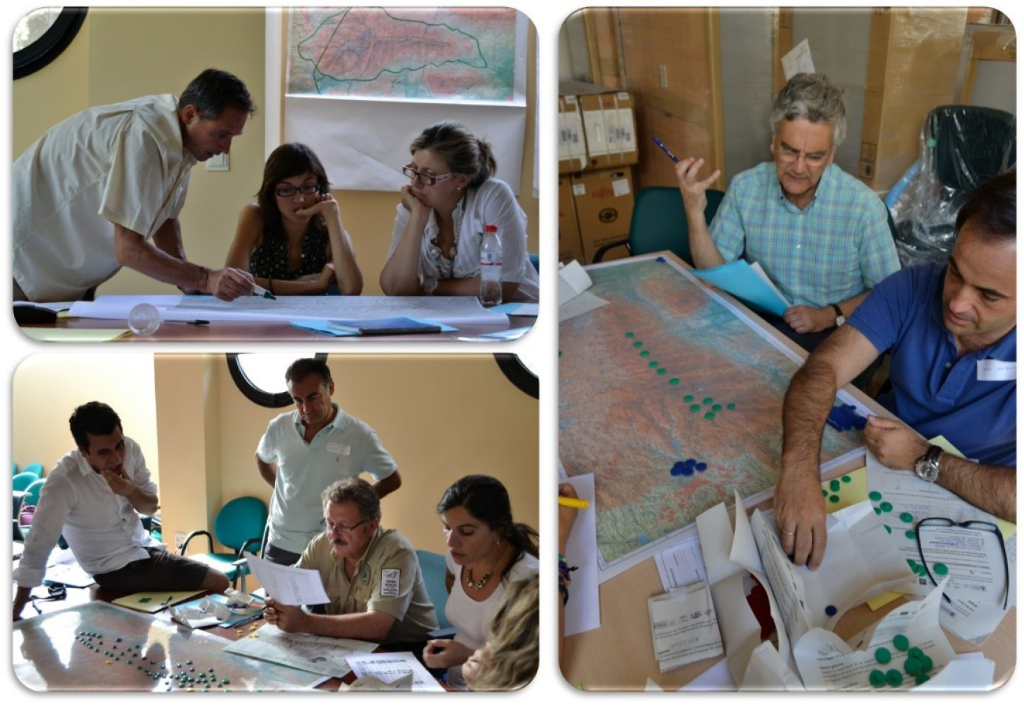
Scenario planning combines various tools and techniques (e.g. interviews, brainstorming or visioning exercises in workshops, often complemented with modelling) to develop plausible and internally consistent descriptions of alternative futures, where values of ES can be elicited. Assumptions about future events or trends are questioned and uncertainties are made explicit to establish transparent links between changes in ES and human well-being.
Deliberative methods comprise various tools and techniques to engage and empower non-scientific participants. These methods (e.g. valuation workshops, citizens' juries, photo-voice, etc.) invite stakeholders and citizens to form their preferences for ES together through an open dialogue. Deliberative methods can address ethical beliefs, moral commitments and social norms and are often used in combination with other approaches (e.g. mapping or monetary valuation).
Scrutiny of specific socio-cultural valuation methods
The diversity of socio-cultural methods described above is determined by different methodological requirements (Table
Methodological requirements of socio-cultural methods for valuing ES. Methods are evaluated according to their suitability to value ES at different spatial scales and to uncover quantitative or qualitative data -(***) high , (**) moderate , (*) low - and according to the level of requirements in terms of data, collaboration, time and economic resources -(H) high , (M) medium , (L) low -. Source: Kelemen et al. (2015).
| SOCIO-CULTURAL METHODS | SPATIAL SCALE | DATA | COLLABORATION | RESOURCES | |||||||
|
Local
|
Regional
|
National
|
Amount of data
|
Qualitative
|
Quantitative
|
Researchers' own field
|
Researchers' other field
|
Non-academic stakeholders
|
Time
|
Economic
|
|
| Preference assessment | *** | *** | * | H | ** | *** | H | H | L | M | M |
| Time use | *** | *** | * | H | * | *** | H | M | L | M | M |
| Photo-elicitation surveys | *** | *** | * | H | ** | *** | H | H | L | M | M |
| Narratives | *** | *** | * | M | *** | ** | L | L | H | M | M |
| Participatory GIS (PGIS) | *** | *** | ** | M | *** | *** | L | H | H | M | M |
| Scenario planning | *** | *** | ** | M | *** | ** | L | H | H | L | M |
| Deliberative valuation | *** | *** | ** | M | *** | *** | L | H | H | M | M |
Main socio-cultural methods are presented in relation to their capacity to integrate different types of values-(***) high , (**) moderate , (*) low, (-) not appropriate - and according to their capacity to integrate values -(H) high , (M) medium , (L) low -. Source: Kelemen et al. (2015).
| SOCIO-CULTURAL METHODS | IPBES values | TEEB values | Total Economic Value | |||||||||
|
Intrinsic
|
Relational
|
Instrumental
|
Ecological
|
Socio-cultural
|
Monetary
|
Direct use values
|
Indirect use values
|
Existence values
|
Bequest values
|
Option values
|
Integrative Potential
|
|
| Preference assessment | * | ** | ** | * | *** | - | ** | ** | ** | ** | * | M |
| Time use | * | ** | ** | * | ** | * | ** | ** | ** | * | * | M |
| Photo-elicitation surveys | * | * | ** | ** | *** | * | ** | ** | ** | ** | ** | M |
| Narratives | ** | ** | ** | *** | *** | - | - | - | * | * | * | L |
| Participatory GIS (PGIS) | * | *** | * | *** | *** | * | ** | * | *** | *** | ** | H |
| Scenario planning | * | *** | *** | ** | ** | ** | * | ** | ** | *** | *** | H |
| Deliberative valuation | ** | *** | ** | ** | *** | * | * | ** | ** | ** | ** | H |
| Degree of values captured by all methods | L | M | M | M | H | L | L | L | M | M | M | |
PGIS is also the most suitable method to provide spatial outputs, although preference assessment, time use and photo-elicitation may also contribute with spatially explicit results by estimating representative values for different geographical areas. PGIS is particularly suited to identify ecosystem service benefiting areas, i.e. places where use or demand of ES converge (see Chapters 5.2 and 5.6.2).
Despite all developments regarding socio-cultural valuation of ES, the question of how socio-cultural valuation methods can elicit the broad range of values associated with nature is still relatively unexplored. Following the conceptual definitions provided for value categories in the Total Economic Value (TEV), the Economics of Ecosystems and Biodiversity (TEEB) and the IPBES, an integrative approach to socio-cultural valuation methods has the capacity to uncover most of the different value categories (Table
The resulting analyses reflect the extent to which diverse valuation methods capture specific value types or have integrative potential, as well as which set of complementary methods can be applied to capture multiple values.
Internal variability of socio-cultural valuation methods
A key similarity amongst socio-cultural methods is the assumption that values of ES are rooted in individuals and, at the same time, shaped by individuals' social and cultural context. In fact, socio-cultural approaches have the capacity to elicit collective and shared values of ES through participatory and deliberative techniques that go beyond the aggregation of individual preferences. Socio-cultural valuation methods aim at valuing ES in a considered way by discovering the psychological, historical, cultural, social, ecological and political contexts and conditions, as well as social perceptions that shape individually held or commonly shared values.
Variability among methods makes socio-cultural valuation capable of flexible adaptation to specific worldviews and decision contexts. Key aspects of this variability include (Figure
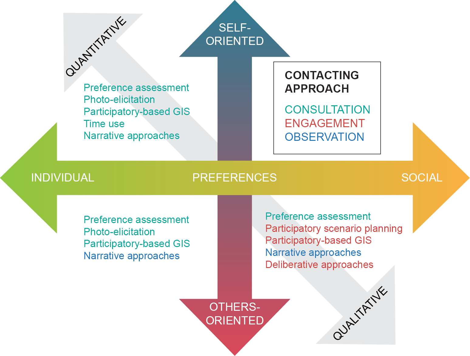
Variability among socio-cultural valuation methods in relation to three axes: type of values elicited, type of rationality attributed to value providers, and the dominant approach of handling data.
1. The type of values elicited: methods focusing on the value to individuals versus methods focusing on the value to society. Values can be considered at the level of the individual (what is considered useful, important, good or morally acceptable by a person) and at higher levels of societal organisation, including a group, a community or the society as a whole (Figure
2. The type of rationality attributed to participants (value providers): self-oriented versus others-oriented methodological approaches. We can distinguish between individual (I) and collective (We) rationality as the two main rules of thumb behind reasonable actions (Figure
3. The process of including participants (value providers) in valuation: observation, consultation or engagement methods. There are three options to gain knowledge on preferences, depending on whether preferences (values) are considered as pre-existing or in the process of formation. Preferences can be observed and reported when participants have a direct relation with the subject of valuation (e.g. they frequently use or enjoy some ES). However, not having a direct relation with the subject of valuation does not necessarily mean that participants do not attribute value to it. To explore these social preferences, participants can be consulted or asked via questionnaires or interviews about their perceptions of ES. If preferences are not expected to exist a priori, or are in the process of formation (i.e. participants do not have a priori knowledge about, or have not faced others' perceptions of certain ES), we can also engage participants in a joint preference formation process through deliberative valuation, participatory scenario planning or PGIS.
4. The dominant approaches to handling data: predominantly quantitative, predominantly qualitative and mixed methodological approaches. All three types of methods can be used to collect quantitative, as well as qualitative data. Quantitative data can be collected in numerical form from large populations and, if representative, can provide results that are applied, in a general sense, from local to regional or even broader spatial scales. Quantitative data can be collected both at individual and group level and then aggregated to generalise the results from the sample to larger populations. Qualitative data allow an in-depth understanding of values and underlying motivations, but usually for a much smaller (and often non-representative) sample. Qualitative data can be collected at the individual and group level in the form of narrative arguments (mainly words, but also pictures, drawings, etc.). Due to the heterogeneity of types of data, aggregation is often impossible and other means of synthesis have to be used (e.g. narrative methods or deliberation). In practice, quantitative and qualitative approaches can be placed along a continuum (Figure
Implementation of socio-cultural valuation methods in the decision-support
Ecosystem service assessments have increasingly been called to support environmental planning, mainly based on biophysical and economic indicators. However, the expectations of decision-makers in relation to how these assessments can support decision-making are not always fulfilled. Moreover, few studies have included the socio-cultural dimension of ES, despite its being considered a research priority. Overlooking the socio-cultural dimension might obscure human-nature relationships and hinder the mainstreaming of ES across societal sectors and in decision-support.
Integrated valuation aims to clarify the interdependencies between the multiple values associated with different ES (see also Box 2 for an example). The biophysical dimension, i.e. an ecosystem's capacity to supply services, determines the range of potential uses by society which also influences its socio-cultural and monetary values. Socio-cultural values might also have an influence on monetary values because individual and social motivations determine the 'utility' a person obtains from a particular service. Conversely, monetary values have social interpretations and the process of monetary valuation is value-articulating in itself. These interdependencies between value dimensions and the different information provided by them, justify combining the different value domains to properly inform environmental decision-making processes.
The major aim of this ES study was to help local stakeholders and decision-makers move towards a more sustainable landscape management system. To this end, in-depth and semi-structured interviews and focus groups were applied. We carried out narrative methods to understand the institutionalised mechanisms affecting farmers' choices that are often in conflict with nature conservation.
Moreover, we carried out deliberative valuation to understand how farmers relate to biodiversity and whether it has different meanings and values to different groups of farmers. A preference assessment survey was carried out to mobilise community members and collect information on their knowledge, opinion and feelings related to ES. This was then channelled into a participatory scenario planning process, combined with modelling, to enable stakeholders and experts to explore alternative future options and choose the most desirable one(s) together. This long lasting research process was able to highlight multiple dependencies between local inhabitants and their surrounding environment. We could identify plural and heterogeneous values and their possible changes across time and space.
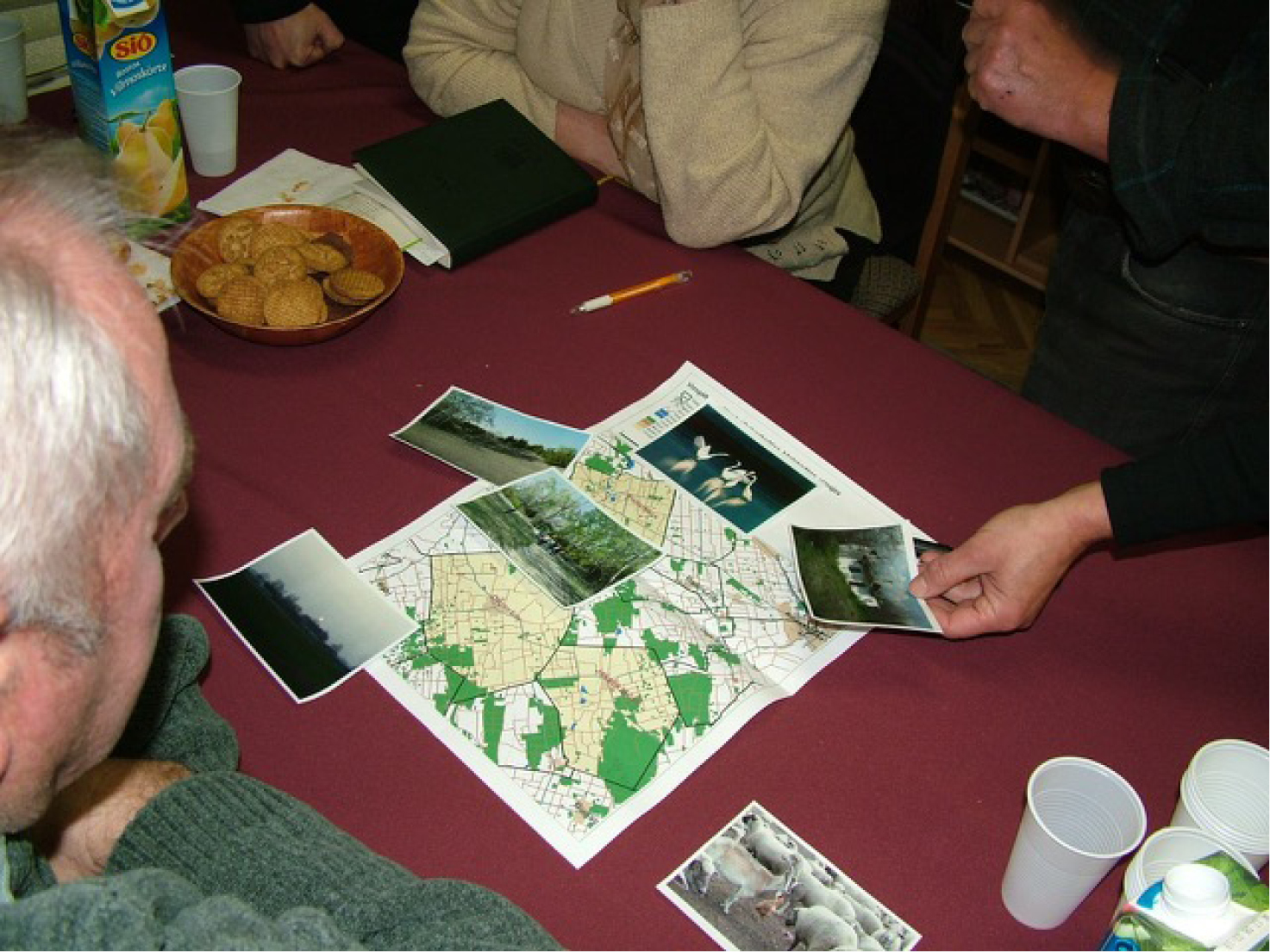
In this section, we formulate several propositions regarding how socio-cultural valuation methods can provide support in decision-making:
1. Socio-cultural approaches help broaden the valuation scope and capture multiple values that complement other valuation methods. Socio-cultural valuation methods can be used to identify how values and perceptions toward ES differ among stakeholders and offer insights into the motivations for conserving nature and the symbolic, cultural and spiritual values that are frequently invisible in other valuation approaches. Further, socio-cultural valuation methods can address relational values that are preferences, principles and virtues associated with nature-human relationships. For example, deliberative methods allow the consideration of ethical beliefs, moral commitments and social norms.
2. Socio-cultural valuation methods can cover different spatial scales. Values derived from large representative samples of a population can be transferred to other locations when the social, cultural and ecological conditions are similar and aggregated to larger scales than the original study. Given the emphasis of socio-cultural valuation methods on social formation and context-dependency of values, some approaches such as value transfer, aggregation and scaling are less common than in economic valuation where assumptions of pre-existing individual preferences encourage comparisons across contexts. In addition, a number of socio-cultural valuation methods are applied at local scales to assess certain values in depth.
3. Socio-cultural valuation methods are a useful tool to identify how plural values are interlinked. These help identify plural and heterogeneous values that are relevant for different people (e.g. different socio-demographic profiles, different cultures or cosmologies), at different temporal scales (e.g. seasons of the year) and different choice situations (individual versus group). Socio-cultural valuation methods can reveal how plural and heterogeneous values are interlinked and contribute to human wellbeing.
4. Socio-cultural methods are more appropriate in situations of social conflict than other valuation methods. Aiming for an in-depth understanding of human-nature relationships, some socio-cultural methods integrate different forms of knowledge (e.g. expert or technical knowledge and experiential and local knowledge) held by different social actors. Sometimes, the interests of one stakeholder group might be in conflict with the interests of other stakeholders and power relations might operate between them. In that case, socio-cultural valuation can support the identification of conflicts arising from different perceptions, needs and uses of ES, as well as power inequities in the access to ES.
5. Socio-cultural preferences can serve as indicators of the impact of different management options on the ecosystems' capacity to deliver services. Socio-cultural preferences are often associated with ecosystem service bundles. They are helpful in identifying ecosystem service synergies and trade-offs resulting from stakeholders' diverging interests and knowledge. Social preferences for ES can be used as indicators of present and future pressures on landscapes and land-use change. For example, multi-criteria analysis can combine a biophysical ecosystem service assessment with people's willingness to trade off one ecosystem service for another, establishing a ranking order of landscape management alternatives that can be used in priority-setting.
In summary, socio-cultural valuation methods can provide decision-support in the form of awareness-raising, value and knowledge recognition, value conflict identification and priority-setting. They also help bring different voices and stakeholders into the decision-making process.
Further reading
- Chan K, Balvanera P, Benessaiah K, Chapman M, Diaz S, Gomez-Baggethun E, Gould R, Hannahs N, Jax K, Klain S, Luck G, Martin-Lopez B, Muraca B, Norton B, Ott K, Pascual U, Satterfield T, Tadaki M, Taggart J, Turner NJ (2016) Why Protect Nature? Rethinking Values and the Environment. PNAS 113: 1462-1465.
- Garcia-Llorente M, Martin-Lopez B, Iniesta-Arandia I, Lopez-Santiago CA, Aguilera PA, Montes C (2012) The role of multi- functionality in social preferences toward semi-arid rural landscapes: an ecosystem service approach. Environmental Science and Policy 19-20: 136-146.
- Gomez-Baggethun E, Martin-Lopez B (2015) Ecological Economics perspective in ecosystem services valuation. In: Martinez-Alier J, Muradian R (Eds) Handbook of Ecological Economics, 260-282. Edward Elgar, London.
- Iniesta-Arandia I, Garcia-Llorente M, Aguilera P, Montes C, Martin-Lopez B (2014) Socio-cultural valuation of ecosystem services: uncovering the links between values, drivers of change and human well-being. Ecological Economics 108: 36-48.
- IPBES (2015) Preliminary guide regarding diverse conceptualisation of multiple values of nature and its benefits, including biodiversity and ecosystem functions and services, IPBES 15 Deliverable 3 (d).
- Kelemen E, Garcia-Llorente M, Pataki G, Martin-Lopez B, Gomez-Baggethun E (2014) Non-monetary techniques for the valuation of ecosystem services. OpenNESS Syntehsis Papers No. 6.
- Kenter J, O'Brien L, Hockley N, Ravenscroft N, Fazey I, Irvine K, Reed M, Christie M, Brady E, Bryce R and Church A (2015) What are shared and social values of ecosystems? Ecological Economics, 111: 86-99.
- Kovacs E, Kelemen E, Kaloczkai A, Margoczi K, Pataki G, Gebert J, Malovics G, Balazs B, Roboz A, Kovacs E, Mihok B (2015) Understanding the links between ecosystem service trade-offs and conflicts in protected areas. Ecosystem Services 12: 117-127.
- Martin-Lopez B, Iniesta-Arandia I, Garcia-Llorente M, Palomo I, Casado-Arzuaga I, Del Amo DDG, Gomez-Baggethun E, Oteros-Rozas E, Palacios-Agundez I, Willaarts B, Gonzalez JA, Santos-Martin F, Onaindia M, Lopez-Santiago C, Montes C (2012) Uncovering ecosystem service bundles through social preferences. PLoS ONE 7(6): e38970.
- Oteros-Rozas E, Martin-Lopez B, Gonzalez JA, Plieninger T, Lopez CA, Montes C. (2014) Socio-cultural valuation of ecosystem services in a transhumance social-ecological network. Regional Environmental Change 14: 1269-1289.
- Plieninger T, Bieling C, Ohnesorge B, Schaich H, Schleyer C, Wolff F (2013) Exploring futures of ecosystem services in cultural landscapes through participatory scenario development in the Swabian Alb, Germany. Ecological and Society 18(3): 39.
- Santos-Martin F, Martin-Lopez B, Garcia-Llorente M, Aguado M, Benayas J, Montes C (2013) Unravelling the Relationships between Ecosystems and Human Wellbeing in Spain. PLoS One 8: e73249.
- Teddlie C, Tashakkori A (Eds) (2009) Foundations of mixed methods research: Integrating quantitative and qualitative approaches in the social and behavioural sciences. Sage Publications Inc.
4.3. Economic quantification
Introduction
Economic quantification of ES attempts to measure the human welfare derived from the use or consumption of ES. Economic quantification or valuation is one way to assess and communicate the importance of ES to decision-makers and can be used in combination with other forms of information (e.g. bio-physical or social quantification - see Chapters 4.1 and 4.2). The comparative advantage of economic valuation is that it conveys the importance of ES directly in terms of human welfare and uses a common unit of account (i.e. money) so that values can be directly compared across ES and across other goods and services that are consumed by society.
The aim of this chapter is to introduce the key concepts underlying economic quantification of ES and to provide an explanation for the various economic methods that can be applied.
The economic value of ES
In this section, we provide definitions of the various concepts of economic value that may be encountered when quantifying ES.
In neo-classical welfare economics, the economic value of goods or services is the wellbeing derived from its production and consumption, usually measured in monetary units. In a perfectly functioning market, the economic value of goods or services is determined by the demand for and supply of those goods or services. Demand for goods or services is driven by the benefit, utility or welfare that consumers derive from it. Supply of goods or services is determined by the cost to producers of producing it. The left-hand panel in Figure
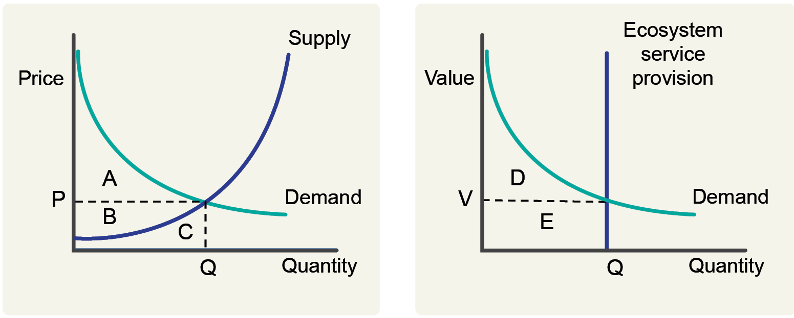
It is important to recognise that, when we make a decision to allocate resources to produce particular goods or services, we are also deciding not to allocate those resources to produce alternative goods or services. The goods or services that we give up is called the "opportunity cost" of our decision. Opportunity cost can be defined as the value of the foregone next best use of resources. This is an important concept in the context of ES since it is often the value of the alternative use of resources (e.g. agriculture, timber extraction, aquaculture) that drives ecosystem loss.
In the case that ES are not traded in a market, the interpretation of the welfare derived from their provision can also be represented in terms of surplus. The right-hand panel of Figure
Total Economic Value
The concept of Total Economic Value (TEV) of an ecosystem is used to describe the comprehensive set of utilitarian values derived from it. This concept is useful for identifying the different types of value that an ecosystem provides. TEV comprises of use values and non-use values. Use values are the benefits that are derived from some physical use of the resource. Direct use values may derive from on-site extraction of resources (e.g. fuel wood) or non-consumptive activities (e.g. recreation). Indirect use values are derived from off-site services that are related to the resource (e.g. downstream flood control, climate regulation). The option value is the value that people place on maintaining the option to use an ecosystem resource in the future given the uncertainty that they would actually use it. Non-use values are derived from the knowledge that an ecosystem is maintained without regard to any current or future personal use. Non-use values may be related to altruism (maintaining an ecosystem for others), bequest (for future generations) and existence (preservation unrelated to any human use) motivations. The constituent components of TEV are represented in Figure
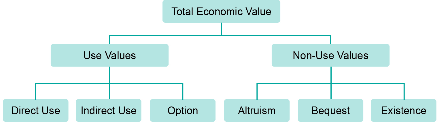
Exchange value
The concept of welfare value is used in most economic assessments of ES but it is not used in the system of national accounts (SNA) that is used to calculate gross domestic product (GDP) and other economic statistics. The SNA uses the concept of exchange value which is a measure of producer surplus plus the costs of production. In the left-hand panel of Figure
The differences between the concepts of welfare value and exchange value are the inclusion of consumer surplus (A) in the former and the inclusion of production costs in the latter (C). The concept of welfare value corresponds to a theoretically valid measure of welfare in the sense that a change in value represents a change in welfare for the producers and/or consumers of the goods and services under consideration. The concept of exchange value does not correspond to a theoretically valid measure of welfare and a change in exchange value does not necessarily represent a change in welfare for either producers or consumers.
Quantifying economic values
A variety of methods have been developed for quantifying the economic value of ES. These valuation methods are designed to span the range of valuation challenges raised by the application of economic analyses to the complexity of the natural environment. An important distinction exists between methods that produce new or original information generally using primary data (primary valuation methods) and those that use existing information in new policy contexts (value transfer methods).
Primary valuation methods
Table
Primary economic valuation methods.
| Valuation method | Approach | Application to ES | Example ecosystem service |
|---|---|---|---|
| Market prices | Prices for ES that are directly observed in markets. | ES that are traded directly in markets. | Timber and fuel wood from forests; Recreation at national parks that charge an entrance fee. |
| Public pricing | Public expenditure or monetary incentives (taxes/subsidies) for ES as an indicator of value. | ES for which there are public expenditures. | Watershed protection to provide drinking water; Purchase of land for protected areas. |
| Defensive expenditure | Expenditure on protection of ecosystems. | ES from protected ecosystems. | Nutrient filtration by protected wetlands |
| Replacement cost | Estimate the cost of replacing an ES with a man-made service. | ES that have a man-made equivalent. | Coastal protection by dunes; water storage and filtration by wetlands. |
| Restoration cost | Estimate cost of restoring degraded ecosystems to ensure provision of ES. | Any ES that can be provided by restored ecosystems. | Coastal protection by dunes; water storage and filtration by wetlands. |
| Damage cost avoided | Estimate damage avoided due to ecosystem service. | Ecosystems that provide storm or flood protection to houses or other assets. | Coastal protection by dunes; river flow control by wetlands. |
| Net factor income | Revenue from sales of environment-related good minus cost of other inputs. | Ecosystems that provide an input in the production of marketed goods. | Filtration of water by wetlands; commercial fisheries supported by coastal wetlands. |
| Production function | Statistical estimation of production function for marketed goods including an ES input. | Ecosystems that provide an input in the production of marketed goods. | Soil quality or water quality as an input to agricultural production. |
| Hedonic pricing | Estimate influence of environmental characteristics on price of marketed goods. | Environmental characteristics that vary across goods (usually houses). | Urban open space; air quality. |
| Travel cost | Use data on travel costs and visit rates to estimate demand for recreation sites. | Recreation sites | Outdoor open access recreation. |
| Contingent valuation | Ask people to state their willingness to pay for an ES through surveys. | All ES | Species loss; natural areas; air quality; water quality landscape aesthetics. |
| Choice modelling | Ask people to make trade-offs between ES and other goods to elicit willingness to pay. | All ES | Species loss; natural areas; air quality; water quality; landscape aesthetics. |
| Group / participatory valuation | Ask groups of stakeholders to state their willingness to pay for an ES through group discussion. | All ES | Species loss; natural areas; air quality; water quality; landscape aesthetics. |
Value transfer methods
Decision-making often requires information quickly and at low cost. New 'primary' valuation research, however, is generally time consuming and expensive. For this reason, there is interest in using information from existing primary valuation studies to make inform decisions regarding impacts on ecosystems that are of current interest. This transfer of value information from one context to another is called value transfer. Value transfer is the use of research results from existing primary studies at one or more sites or policy contexts ("study sites") to predict welfare estimates or related information for other sites or policy contexts ("policy sites"). Value transfer is also known as benefit transfer but since the values that are transferred may be costs as well as benefits, the term value transfer is more generally applicable.
In addition to the need for expeditious and inexpensive information, there is often a need for information on the value of ES at a different geographic scale from that for which primary valuation studies have been conducted. So, even in cases where some primary valuation research is available for the ecosystem of interest, it is often necessary to extrapolate or scale-up this information to a larger area or to multiple ecosystems in the region or country. Primary valuation studies tend to be conducted for specific ecosystems at a local scale whereas the information required for decision-making is often needed at a regional or national scale. Value transfer therefore provides the means to obtain information for the scale that is required.
The number of primary studies on the value of ES is substantial and growing rapidly. This means that there is a growing body of evidence to draw on for the purposes of transferring values for informed decision-making. With an expanding information base, the potential for using value transfer is improved.
Value transfer can potentially be used to estimate values for any ecosystem service, provided that there are primary valuations of that ecosystem service from which to transfer values. The use of value transfer is widespread but requires careful application. The alternative methods of conducting value transfer are described here.
Unit value transfer uses values for ES at a study site, expressed as a value per unit (usually per unit of area or per beneficiary), combined with information on the quantity of units at the policy site to estimate policy site values. Unit values from the study site are multiplied by the number of units at the policy site. Unit values can be adjusted to reflect differences between the study and policy sites (e.g. income and price levels).
Value function transfer uses a value function estimated for an individual study site in conjunction with information on parameter values for the policy site to calculate the value of an ecosystem service at the policy site. A value function is an equation that relates the value of an ecosystem service to the characteristics of the ecosystem and the beneficiaries of the ecosystem service. Value functions can be estimated from a number of primary valuation methods including hedonic pricing, travel cost, production function, contingent valuation and choice experiments.
Meta-analytic function transfer uses a value function estimated from the results of multiple primary studies representing multiple study sites in conjunction with information on parameter values for the policy site to calculate the value of an ecosystem service at the policy site. A value function is an equation that relates the value of an ecosystem service to the characteristics of the ecosystem and the beneficiaries of the ecosystem service. Since the value function is estimated from the results of multiple studies, it is able to represent and control for greater variation in the characteristics of ecosystems, beneficiaries and other contextual characteristics. This feature of meta-analytic function transfer provides a means to account for simultaneous changes in the stock of ecosystems when estimating economic values for ES (i.e. the "scaling up problem"). By including an explanatory variable in the data describing each "study site" that measures the scarcity of other ecosystems in the vicinity of the "study site", it is possible to estimate a quantified relationship between scarcity and ecosystem service value. This parameter can then be used to account for changes in ecosystem scarcity when conducting value transfers at large geographic scales.
These three principal methods for transferring ecosystem service values are summarised in Table
Value transfer methods.
| Approach | Strengths | Weaknesses | |
|---|---|---|---|
| Unit value transfer | Select appropriate values from existing primary valuation studies for similar ecosystems and socio-economic contexts. Adjust unit values to reflect differences between study and policy sites (usually for income and price levels). | Simple | Unlikely to be able to account for all factors that determine differences in values between study and policy sites. Value information for highly similar sites is rarely available. |
|
Value function transfer |
Use a value function derived from a primary valuation study to estimate ES values at policy site(s). | Allows differences between study and policy sites to be controlled for (e.g. differences in population characteristics). | Requires detailed information on the characteristics of policy site(s). |
| Meta-analytic function transfer | Use a value function estimated from the results of multiple primary studies to estimate ES values at policy site(s). | Allows differences between study and policy sites to be controlled for (e.g. differences in population characteristics, area of ecosystem, abundance of substitutes etc.). Practical for consistently valuing large numbers of policy sites. | Requires detailed information on the characteristics of policy site(s). Analytically complex. |
Representing economic values on maps
The representation of economic values on maps involves estimating variable combinations of supply and demand across spatial units and plotting the resulting values. Spatial units in a value map can include land parcels (e.g. polygons representing ownership), ecosystem patches (e.g. polygons representing distinct ecosystems of different type), ecosystem units (e.g. raster grids of ecosystem type), grid cells (e.g. raster grids with land use/land cover), or beneficiaries (e.g. people plotted using residential or activity location). In most cases, spatial units are used to represent the ecosystem that supplies the ecosystem service, but mapping values by the location of beneficiaries can be useful in some decision-making contexts (e.g. for representing the distributional consequences of changes in ecosystem service provision across communities; or for designing payment mechanisms for ES).
In mapping ecosystem service values, each spatial unit is treated as a separate sub-market for the ecosystem service. Methods for mapping ecosystem service values can address spatial variations in supply, demand, or a combination of both determinants.
general terms, bio-physical methods (see Chapter 4.1) are used to estimate the spatially variable quantities of ES supplied (e.g. probability of flood damage, quantity of clean water, area of recreational space, tonnes of carbon stored) and economic methods are used to estimate spatially variable marginal values per unit of ecosystem service provided and consumed. Mapping economic values therefore necessarily involves linking maps of biophysical ecosystem supply with economic valuation methods.
Production/consumption statistics
In addition to the quantification of human welfare derived from ES in monetary units, economic quantification of ES encompasses the recording or estimation of production and consumption statistics in physical units. Indeed, the measurement of physical units of production and consumption of ES is a necessary a step in the process of quantifying economic value. Economic quantification may, however, stop short of estimating values and directly report production and consumption statistics as useful information to support decision-making.
To a great extent, the production of ES is quantified using bio-physical methods (see Chapter 4.1). For most ES, however, it is also necessary to use insights and methods from economics to measure the quantities that are actually used (i.e. to quantify utilised services as opposed to potential services). This generally involves measuring the extent of demand for ES in terms of the population and preferences of beneficiaries.
The physical units in which production and consumption statistics are reported are specific to each ecosystem service. For example, non-timber forest products (NTFPs), such as wild honey, may be measured in kilograms; water extracted for consumption is measured in kilolitres or megalitres, carbon sequestration is conventionally measured in tonnes of carbon or CO2; and recreational use of natural open space may be measured in numbers of visits - all usually expressed per unit of time over which the flow of service is recorded (e.g. per year). In very few cases will the quantity of an ecosystem service be explicitly observed and recorded in a systematic and accessible way (i.e. there is generally not an equivalent of the business activity surveys conducted for the SNA). In most cases, it is necessary to estimate the level of production and consumption using some form of bio-economic modelling.
Freshwater ecosystems provide a variety of ES that can be affected by changes in water quality. In this case study, projected future changes in water quality for the period 2000-2050 are quantified using the IMAGE-GLOBIO model. This information is combined with a meta-analytic value function to estimate the economic value of changes in water quality. The analysis is performed at the resolution of 50 km grid cells. The supply of ES from water bodies (rivers and lakes) is implicitly modelled within the meta-analytic value function. The results of this value transfer application are mapped in order to communicate the spatial distribution of benefits (losses) derived from improvements (declines) in water quality (see Figure
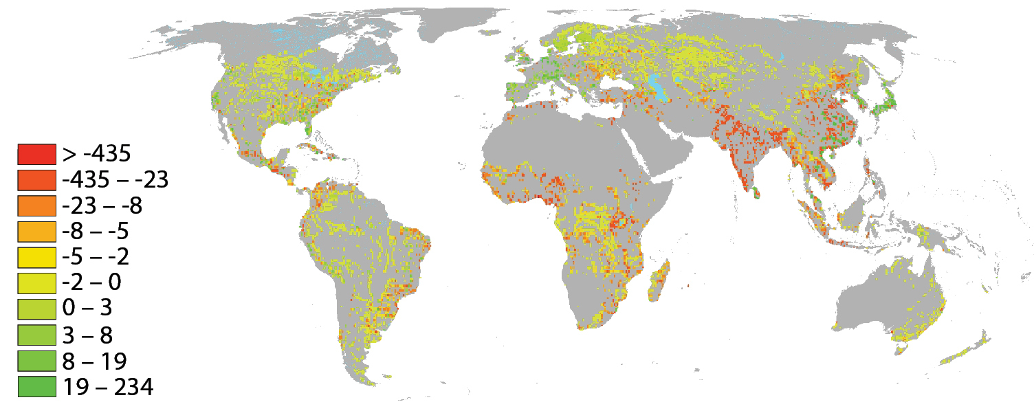
The regulating service of carbon sequestration by ecosystems represents a special case in which supply is spatially variable (dependent on vegetation type, soil characteristics etc.) but demand is entirely spatially disconnected (since CO2 is a uniformly mixing stock pollutant, the marginal benefit of sequestration is not related to where the sequestration takes place). Figure
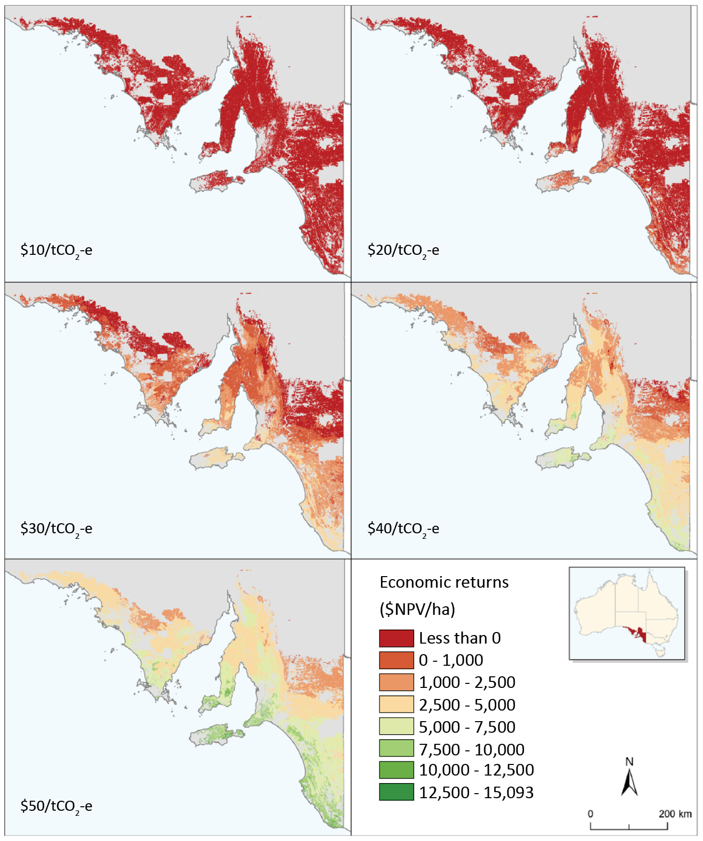
This case study provides an example of how bio-physical and economic modelling can be combined to quantify production statistics for a provisioning ecosystem service. The production of non-timber forest products (NTFPs) in Mondulkiri province, Cambodia, is quantified by combining a validated biophysical model (InVEST) of NTFP availability with an economic model of household decisions regarding the number of harvesting trips to be undertaken and a separate economic model of harvest yield per trip. The bio-physical model quantifies the availability of six NTFPs given spatial variation in forest cover and species diversity. The harvest-trip function, estimated using data from a household survey, quantifies how many trips each household makes given their income, household size and the availability of NTFPs within harvesting distance of their village. The harvest yield function, also estimated using data from a household survey, quantifies how much of each NTFP is harvested per trip given household characteristics, number of trips made and NTFP availability. Figure
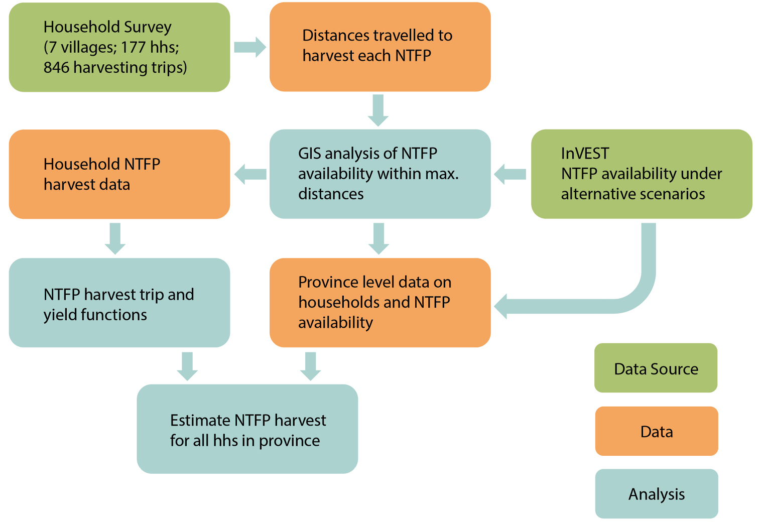
Further reading
- Bagstad KJ, Johnson GW, Voigt B, Villa F (2013) Spatial dynamics of ecosystem service flows: a comprehensive approach to quantifying actual services. Ecosystem Services 4: 117-125.
- Bouma JA, van Beukering PJH (Eds) (2015) Ecosystem Services: From Concept to Practice. Cambridge University Press.
- Brander LM, Brauer I, Gerdes H, Ghermandi A, Kuik O, Markandya A, Navrud S, Nunes PALD, Schaafsma M, Vos H, Wagtendonk A (2012) Using meta-analysis and GIS for value transfer and scaling up: Valuing climate change induced losses of European wetlands. Environmental and Resource Economics 52: 395-413.
- Brander LM (2013) Guidance manual on value transfer methods for Ecosystem Services. United Nations Environment Programme. ISBN 978-92-807-3362-4.
- Brander LM (2015) . Economic valuation of Ecosystem Services in the Eastern Plains Landscape, Modulkiri, Cambodia. Report for WWF Cambodia.
- Brouwer R et al. (2009) Economic Valuation of Environmental and Resource Costs and Benefits in the Water Framework Directive: Technical Guidelines for Practitioners. AquaMoney.
- Bryan BA, Crossman ND (2013) Impact of multiple interacting financial incentives on land use change and the supply of Ecosystem Services. Ecosystem Services 4: 60-72.
- DEFRA (2013) Guidance for policy and decision makers on using an ecosystems approach and valuing Ecosystem Services. Department for Environment, Food & Rural Affairs https://www.gov.uk/ecosystems-services.
- DEFRA (2007) An introductory guide to valuing Ecosystem Services (2007) Department for Environment, Food and Rural Affairs.
- Freeman AMI (2003) The Measurement of Environmental and Resource Values. Resources for the Future, Washington D.C.
- Johnston RJ, Rolfe J, Rosenberger RS, Brouwer R (Eds) (2015) Benefit transfer of environmental and resource values: A handbook for researchers and practitioners. Springer. ISBN 978-94-017-9929-4.
- Pascual U, Muradian R, Brander L, Gomez-Baggethun E, Martin-Lopez B, Verma M (2010) The economics of valuing Ecosystem Services and biodiversity. In Kumar (Ed.) The Economics of Ecosystems and Biodiversity: Ecological and Economic Foundations. Earthscan, London and Washington.
- Pearce D et al. (2001) Economic Valuation with Stated Preference Techniques Summary Guide. Department of Transport, Local Government and Regions, London.
- Schagner JP, Brander LM, Maes J, Hartje V (2013) Mapping ecosystem service values: Current practice and future prospects. Ecosystem Services 4: 33-46.
4.4. Computer modelling for ecosystem service assessment
Introduction
Computer models are simplified representations of the environment that allow biophysical, ecological, and/or socio-economic characteristics to be quantified and explored. Modelling approaches differ from mapping approaches (Chapter 5) as (i) they are not forcibly spatial (although many models do produce spatial outputs); (ii) they focus on understanding and quantifying the interactions between different components of social and/or environmental systems and (iii) by changing parameters within models, they are capable of exploring both alternative scenarios and internal model dynamics.
When applied to the assessment of ecosystem services (ES), models are important tools which can quantify the relationships that underpin ES supply, demand and flows and, in some cases, produce maps representing these factors. Furthermore, as models can explore scenarios, trade-offs that result from different scenarios can be assessed. This chapter provides a broad overview of different types of models that have been applied to ES assessments and discusses, with examples, the ways that these models have the potential to be used in practice.
In the context of ES, there are a number of ways of distinguishing between different types of models. Here, we distinguish between individual models focussing on single ES and modelling frameworks that can assess multiple ES within the framework of a single modelling tool.
What is a model
A model is a simplification of reality that represents the relationship between two or more sets of factors and uses one set of factors to predict values of the other: y = x2 is a simple model where the variable y can be predicted from variable x by performing the square function on x. However, there are many different types of models, most of which are considerably more complex.
When used in ES research, models are generally used to predict either ES themselves, or underlying environmental aspects from which ES are derived. ES models use diverse types of input variables, but commonly include measurements of environmental parameters (e.g., tree heights, river flows, species counts), survey responses or scores given by scientists or stakeholders (e.g., from questionnaire responses or interviews) or the outputs from another model (e.g., outputs from a climate model may provide precipitation inputs to a water flow model).
What sorts of models are useful for ES assessment
Computer modelling predates the popularisation of the ES concept and models have a decades-long history of use within the environmental sciences. As such, there are a large number of models that can be used to assist in ES assessment, though older biophysical models may be less deliberately beneficiary-orientated than more modern ES models.
It is beyond the scope of this chapter to provide a full overview of modelling per se. In the following text, we describe five general types of models that are used for ES assessment.
Conceptual models
Conceptual models, although rarely computerised, are the first stage of any computer modelling process. They are used to gain an understanding of linkages between different components of the system being studied. The carbon and water cycles, for example, provide the underlying conceptual models for a number of more detailed computer models used to predict ES, such as carbon sequestration by vegetation or the role of vegetation in mediating floods. The first step of any new computerised modelling process is to draw a conceptual diagram that illustrates how model components interlink, then to determine how to quantify those linkages.
Statistical models
Where there is no known quantified relationship between components of the conceptual model, statistical models can help to establish relationships by drawing on collected data. For example, if a conceptual model suggests that freshwater provisioning is driven by rainfall and forest cover in a catchment area, corresponding data can be collected and regression-based approaches can be used to explore the strength of these relationships. Sufficiently strong relationships that are identified can then be used in a deterministic model to predict expected freshwater provisioning in areas for which data are not present.
Deterministic models
A deterministic model assumes links between cause and effect. The y = x2 example above is a very simple deterministic model: for every example of x the value of y will be x2. Deterministic models are usually based on fundamental physical laws derived from a process-based understanding of the science (e.g., the physical sciences or, as above, a statistically derived relationship).
An implicit implication of deterministic models is that there is only one possible output for a given set of inputs (x2 will always enumerate to x2). This can lead to a false impression of accuracy when modelling complex systems where uncertainty is common. Probabilistic models have emerged to address these issues.
Deterministic models underpin many common ES assessment approaches. The Revised Universal Soil Loss Equation (RUSLE), for example, is a commonly used deterministic model developed to better understand the factors driving soil loss from agricultural land. Expressed as: A = R x K x LS x C x P, it relates soil loss (A) to rainfall erosivity (R), soil erodibility (K), slope steepness and length (LS), management practice (C) and conservation practice (P).
Probabilistic models
Probabilistic models recognise that random behaviour is often part of a system; they express likelihoods of events occurring (e.g., the return period of a flood of a given magnitude). Rather than using single values as inputs, probabilistic approaches use probability distributions functions (PDFs) as input parameters. Instead of using mean rainfall, a probabilistic approach might use a range of inputs sampled from a normal distribution around the mean up to the maximum and minimum recorded observations. These sample values can be selected systematically or randomly (the "Monte Carlo" approach) and then run through a deterministic model to explore the range of outputs that result. This allows the probability of a given output to be assessed, rather than implying that, in a complex system, a single output value can be expected for a given combination of inputs.
Rule-based modelling
Rule-based models can be applied, using Boolean (yes/no) decisions and if-then statements to construct a path from input to output. They are often represented as nested decision trees. These are common in remote sensing and biological classification keys and use if-then options to decide between possible output classes (e.g., if variable x, representing tree cover, is above a given threshold then class y = forest, otherwise class y = grassland). Rule-based models can also be incorporated into context-aware artificial intelligence (AI)-supported model selection platforms that account for context by selecting from a library of possible data and models.
Agent-based models (ABMs) are a special type of rule-based model that set (usually simple) rules for individual "agents." By allowing the individual agents to interact in a model, collective behaviour emerges. The "agents" within an ABM can represent anything from individual species or decision-makers to institutions or countries at international levels. Another important aspect of ABMs is that agents' learning from experience can be simulated within the model as it runs, allowing ABMs to model aspects such as the transfer of ideas between individuals and other organic processes.
The ABM approach is very different from deterministic approaches, where a clear path can be traced between model inputs and outputs. Within an ABM, results depend on the timing, identity and consequences of agents' interactions. If there is an element of randomness in the guiding rules (i.e., 50% of the time an agent makes choice X and 50% choice Y), then the same outcome will not be replicated on repeated model runs although, over a large number of runs, common emergent behaviour may be apparent.
In ES assessment, ABMs offer significant opportunities to understand how interactions between individual actors may influence ES. This could involve human actors (e.g., farmers) interacting with policies and institutional structures to determine the best crop types for their farm and the associated impact of this change for ES provision. Or, it could assess the effects of predator-prey species interactions on the ES provided by these species.
Integrated modelling systems
Models tend to be developed for specific purposes, to address a particular problem raised within a given sector. However, within a single-sectoral model, any number of individual models may be used to represent different linkages within the conceptual model. Furthermore, the outputs of one model may be used to provide inputs to another model creating modelling chains. This can allow integrated modelling systems to be set up that take into consideration cross-sectoral interactions, synergies and trade-offs including, for example, the implications for one ES (e.g., drinking water provision) as a result of changes in another (e.g., soil erosion regulation).
How can models help us better understand ES
The previous section provided a brief overview of the types of models that exist to provide information to help with ES assessment. We next focus on how these models can be used, i.e., on which aspects of the environment do models provide information and how does this help us better assess ES?
In the following sections, we consider four main applications of models. First, models of the natural environment that do not provide direct information about ES, but can assess underlying ecosystem structures and functions from which ES can be understood. Second, models that are focussed on ES, both on individual services and those intended to enable assessment of a suite of different ES. Third, modelling systems that take an integrated approach to ES, which allows for an assessment of trade-offs and synergies between groups of services. Finally, models designed to explore ES with decision-makers or stakeholders.
Models of the natural environment
Many more models address the natural environment than address the more recent field of ES. Such models may need to be extended to evaluate ES. However, as some have been used for many decades, they may be well known, understood and trusted by stakeholders. This may make them useful entry points to introduce the ES concept, or may introduce a barrier of inertia ("we have a tool that works, so why change it?").
Species distribution models, land use/land cover (LULC) models and general biophysical models are common natural systems models that can provide ES assessment.
Species distribution modelling
Species distribution modelling (SDM) is often used to identify how plant and animal species respond to changing environmental parameters such as atmospheric CO2, climate, or habitat availability. There is a wide range of approaches to SDM, such as simple, statistical "profile methods," regression-based techniques and approaches that use machine learning. Advanced SDM approaches combine these maps with land use modelling (see below) to determine where habitats are available and, using dispersal and connectivity models, can project the abilities of species to colonise new habitats.
The outputs of species distribution models are maps of species distributions for a given scenario. These can be used to assess ES provision related to these species. For example, maps of charismatic or endemic species distributions can help assess whether particular areas may maintain or lose species with particular religious, social or cultural value.
Land use/land cover modelling
Land use/land cover data are key inputs to many ES mapping approaches (see Chapter 5) and there are various ways to link LULC with additional datasets to map ES (e.g., the "matrix approach" see Chapter 5.6.4). Initial land cover data are often derived from remote sensing or habitat mapping and land use can be modelled from this baseline in a wide range of ways. Given the impacts of LULC change on ES (i.e., through urbanisation, agricultural intensification, or ecological restoration), LULC data have obvious value in understanding how ecosystem service flows are changing over time. Three common approaches are detailed below.
First, "Lowry-type" models can quantify where the location of an attribute of interest (e.g., demographic data or recreational opportunities) is a function of the attraction and travel costs associated with different locations (using, for example, the Rural Urban Growth model (RUG) or the Ecosystem Service Mapping Tool (ESTIMAP)).
Second, by assigning probabilities to transitions between land use types (for instance, 50% of grassland will turn to forest), transition probability approaches can project land use change into the future. These probabilities can themselves be driven by other spatial and/or scenario variables to produce more complex patterns of change.
Third, state-and-transition models (STMs) are conceptual models that use simple, diagrammatic approaches to address non-linear shifts in ecosystems in response to external environmental or anthropogenic disruption. State-and-transition models are typically created through a consultation process with experts and their diagrammatic approach makes them well suited to participatory work with stakeholders. A STM consists of a recognised number of possible states of an ecosystem and the factors driving transitions between these states. Some, but not all, STMs are spatially explicit.
Finally, agent-based modelling can also be used to understand how interactions between groups of actors and their environment (e.g., individual farmers or policy makers under changing environmental or socio-economic factors) lead to different LULC patterns. Such approaches allow LULC to evolve in response to the agents' changing understanding of the environment as they adapt and learn.
ABMs thus provide a powerful tool for exploring emergent properties in LULC change.
Biophysical models
A large number of biophysical models address major environmental systems, including climatic, ecological, hydrological and geochemical models of key earth systems such as air, soil and water.
Well-known examples include the Soil and Water Assessment Tool (SWAT), which can be used to assess water-related ES and the above-mentioned Revised Universal Soil Loss Equation (RUSLE).
Such models tend to focus on a single aspect of the environment (such as the hydrological, soil, or biological subsystem) and may not be directly appropriate for assessing ES in their strictest sense. Often an additional modelling component will be needed to convert from a biophysical parameter (such as annual soil loss) to its ES (e.g., impacts of soil loss on drinking water quality), particularly to connect these processes to their human beneficiaries. However, due to their long history many of these models are often trusted by environmental decision makers, sometimes making them more preferable than some more recent ES-specific tools.
Modelling systems that explicitly focus on ES
As interest in ES has grown, tools have been developed with an explicit focus on individual ES or suites of services. Some of these tools have been developed to be transferable across contexts whilst others are hard-wired into their local context. In the following sections, we discuss a number of these tools to illustrate broad categories of available approaches and how they are used for ES assessment.
Matrix-based approaches
Matrix-based approaches sit on the border between ES mapping and modelling. They combine GIS (geographical information system) and spreadsheets analysis of LULC input data to produce maps of ES supply and/or demand. At their simplest, these are just mapping techniques (see Chapter 5.6.4 for a more complete description): they combine GIS LULC layers and scored values for the provision of ES to provide ES provision maps across a study area. By using standardised values, ES provision may be compared between regions or, by using locally targeted ES values, more locally appropriate values can be generated. The process can be undertaken with stakeholders to allow maps of both ES supply and demand to be mapped. Additional GIS datasets can be included to improve the processa process known as a multi-attribute lookup tableand these can be modified to reflect management scenarios.
Matrix-based approaches can be applied with very limited technical expertise. However, the more the matrix values rely on expert knowledge rather than quantification with primary data, the more they are open to the critique of over-simplification and subjectivity, particularly when compared to primary data or more detailed modelling approaches. We include this technique here to stress that ES computational modelling need not always be complex.
Transferable ES modelling frameworks
A number of frameworks have been developed with standardised methods designed to be transferred between contexts. Three of the most commonly applied modelling frameworks, InVEST, ESTIMAP and ARIES are described below but there are numerous others (e.g., Co$ting nature, LUCI, MIMES; see Chapter 3.4) and still others which are under development.
InVEST
InVEST (http://www.naturalcapitalproject.org/invest/) is a suite of modelling tools that provides a standard approach for application to varied contexts. InVEST includes 18 tools for assessing marine, coastal, terrestrial and freshwater ES. Each output is spatially explicit and driven by user-input spatial datasets. Most InVEST models account for both ES supply and demand, in terms of the locations of people who would benefit from these services; this allows supply-demand mismatches to be assessed.
InVEST models are freely available and open-source. InVEST requires quantitative skills to be run; although experience with GIS is required to map outputs, coding is not required and the models can be run independently of specialised software (using industry standard or open-source GIS platforms to visualise and prepare input and output data). Collecting and processing the datasets required can take time and effort.
Each of InVEST's tools is a separate model and can be run independently, depending only on the user's needs. The outputs can be produced in biophysical units (i.e., tonne C km-2) or monetised, however the interactions between ES are not specifically modelled.
InVEST has been used in a wide range of contexts including using ES metrics to assess sustainable coastal management in Belize, supporting decision-making over clean water supply in Latin America and national ecosystem planning in China. InVEST is a good example of a suite of tools that has gained ground through its use in multiple contexts. However, it does not yet assess the full range of ES and, like many biophysical models, is weaker on harder-to-assess cultural ES (see Chapter 6.6).
ESTIMAP
ESTIMAP is a collection of spatially explicit modelling approaches that assess the supply, demand and flow of ES. It is implemented within a GIS and is designed to be a standardised, replicable system developed for use in the European Union (EU). It uses different methodologies for some ES and covers different ES than InVEST, focussing mainly on regulating ES (air quality regulation, protection from soil erosion, water retention, pollination, habitat for birds, and recreation). Although the ESTIMAP approach was developed to be applied at the EU scale for policy support, it is quite flexible and can be customised for application to local case studies or specific problems in a way that is more difficult with InVEST's pre-made models.
ARIES
ARtificial Intelligence for ES (ARIES) is a flexible modelling framework that uses AI to select the most appropriate modelling components (deterministic, probabilistic, or ABM) to map ES at context-appropriate scales. This approach moves away from the idea that one model should fit all circumstances. The ARIES framework attempts to recognise the dynamism and complexity of environmental systems and balances this with the need for models that are simple enough to remain usable at a range of spatial scales and in a variety of contexts. ARIES has a strong focus on both the identification of beneficiaries and not oversimplifying ES to static values but instead focusing on dynamic benefits that change with both space and time. It is cloud-based and semantic which allows diverse users to contribute data and models to a growing library that the AI system can select from, increasing its power and flexibility. In other ways, it shares many common attributes with InVEST (i.e., it is spatially explicit, open-source and production function-based).
Integrated assessment models
To combat the fact that many models are focussed on individual ES and may ignore or oversimplify key interactions, integrated assessment models have been developed that link sectoral models in a way that the outputs of one are used as the inputs of another. This approach, though often technically challenging and time consuming to implement, ensures that outputs have taken other sectors into consideration in a way that comparing individual sectoral or ES models for the same scenario cannot. For example, an agricultural model may calculate water availability for irrigation based on rainfall, but without integrating a water allocation model that splits water availability between different sectors (e.g., irrigation, domestic supply, industry or power), it would be impossible to know whether that irrigation water was actually available for use.
There are two main classes of integrated assessment models differentiated predominantly by their application at global or regional scales. An example of each is illustrated below.
GLOBIO-ES
GLOBIO-ES is an example of a dynamic global system model. It is a tool to assess past, present and future impacts of human activities on biodiversity and ES. Impacts on biodiversity are captured in terms of the biodiversity indicator Mean Species Abundance (MSA) and ecosystem extent. Impacts on ES are included for 10 services. The model has been applied at both the national and global scales (see Chapter 5.7.3).
GLOBIO-ES uses cause-effect relationships between environmental variables and ES identified by a literature review. It simulates future changes in ecosystem functions and services on a global scale. The methodology uses spatially explicit inputs on environmental drivers from the global climate and agriculture model IMAGE and the global land use model GLOBIO.
The close link to the IMAGE-GLOBIO framework enables the assessment of interactions between human development (e.g., consumption patterns) and the natural environment (e.g., climate) based on key drivers like population growth, economic development, policy and governance, technology, lifestyle and natural resource availability. The future directions of these drivers are quantified from different scenarios of future socio-economic developments.
CLIMSAVE Integrated Assessment Platform (IAP)
The CLIMSAVE IAP is an example of a regional integrated assessment model. It is a freely accessible web-based model that provides options for ES assessment at a European scale. It is based on an integrated system of models for a number of different sectors including urban growth, freshwater, coastal/fluvial flooding, biodiversity, agriculture and forestry.
The model provides a number of output variables from the integrated models including indicators related to land use and a variety of ES.
A wide selection of climate scenarios is included within the system as well as four stakeholder-defined socio-economic scenarios. The socio-economic input settings are able to be fully customised beyond the pre-set scenarios for a number of socio-economic drivers and adaptation options. This allows the IAP the ability to explore a very broad range of combined socio-economic and climate scenarios to analyse their impacts on ES and allows adaptation options to be explored. This enables ES synergies and trade-offs to be investigated at a European scale.
MIMES (Multiscale Integrated Model of Ecosystem Services)
MIMES is an integrated assessment system that models five distinct 'spheres': the lithosphere, the hydrosphere, the atmosphere, the biosphere and the anthroposphere. Interactions between spheres are controlled using a matrix and ES are modelled by applying production functions that link ES to the system elements necessary to produce those services. Demand profiles, created for different societal groups are used to determine how environmental processes lead to production and use of ES. MIMES is also designed to assist in learning about system processes and the broad range of possible futures rather than providing definitive maps of expected futures. However, whereas CLIMSAVE uses interlinked process-based models, MIMES takes an approach using production functions linked to an economic input-output model.
Models to help with decision-making
The ES concept provides decision-makers with a different way of looking at environmental management problems. A forest is no longer just a timber stock, but also a provider of climate regulation, habitat provision, scenic beauty and recreation. Whilst this brings a broader lens to the value of ecosystems, it also brings new challenges: how do we decide which ES are more important? What are the implications if we choose to harvest the forest as timber?
Modelling can help provide quantitative answers to many of these questions. In the following sections, we provide examples of how modelling can help decision-makers explore the implications of management alternatives. The line between previously mentioned modelling tools and the decision support elements, discussed below, is somewhat fuzzy and we recognise that previously mentioned models and modelling tools can be integrated with the approaches that follow.
Bayesian Belief Networks (BBNs)
A Bayesian Belief Network is a type of model that uses conditional probability to assign likelihoods to a suite of potential outputs given a known state of some or all of the inputs (see Chapter 4.5 for more information about Bayesian Belief Networks).
When applied to ES, BBN inputs are likely to be factors determining ES supply (such as land cover, soil types and other environmental parameters) whilst the outputs will be ES supply, demand costs or benefits.
BBNs have a number of advantages. First, they are very flexible in terms of the data that they can integrate. Both qualitative and quantitative values can be used, allowing them to be populated from field data, outputs from other models and expert opinion. They are also capable of integrating more complex models within them. Second, if the conditional probabilities are not known, they can be inferred from existing data using automated machine learning or a statistical approach. Third, their conditional probabilistic approach explicitly takes uncertainty into consideration so that neither inputs nor outputs are forcibly treated as a deterministic single value. Fourth, BBNs can be embedded in a GIS or web-based platform to provide outputs that can be demonstrated spatially. Finally, they are well suited for exploring scenarios interactively with stakeholders as the modification of inputs allows for a quick identification of changing probabilities of the outcomes which can be performed directly with stakeholders.
Multi-Criteria Decision Analysis (MCDA)
Multi-criteria decision analysis is an umbrella term for a suite of flexible modelling approaches designed to highlight the optimal choice in a situation with many decision alternatives. It breaks problems down into smaller components and analyses and values these relative to one another in terms of a number of consequences (e.g. costs, ecological and social impacts).
When applied to ES assessment, MCDA can be used to evaluate trade-offs between multiple ES in a variety of different scenarios. MCDA is explicitly designed as a decision support tool and has been used with both individual decision makers and groups of stakeholders to analyse preferences for different decision outcomes.
Participatory modelling with stakeholders
Modelling has traditionally been performed by experts in isolation from decision-makers and stakeholders. This has led to criticisms of elitism and has been shown to reduce stakeholder interest, understanding and trust in the modelling. Including stakeholders in the modelling process has, however, been demonstrated to increase the legitimacy of the modelling in the eyes of the stakeholders. Furthermore, taking the stakeholder's local knowledge into consideration often improves the quality of the modelling itself (see Chapter 4.6).
In an ES context, the importance of particular ES to local people can be paramount to their overall value. Participatory modelling ensures that the modelling performed highlights ES that are of most importance to the local context rather than addressing a standard suite of service outputs that miss locally important ES.
A "knowledge co-production" approach can be taken with any modelling approach which places interactions between the modeller and stakeholder on an even ground. Due to their iterative nature, such approaches are often considerably more time- consuming. In fact, it may require modellers to develop entirely new models to address questions posed by stakeholders rather than the questions they pose themselves. This may mean that approaches which modellers would have planned to follow (e.g. expanding existing models) may not be appropriate for addressing stakeholder needs.
Considerations with modelling ES
We conclude by discussing five general issues that should be considered when modelling ES.
Which ES
Not all ES are as easy to model as others. In general, provisioning and regulating services have a longer history of being modelled than cultural ES. In fact, modelling cultural ES tends to be limited to analyses of services with relatively tangible physical aspects to their provision, such as recreation, tourism and, to some extent, aesthetic beauty. This is because factors with greater social or cultural meaning are considerably harder to tie to environmental parameters. It is in situations such as these that participatory approaches come to the fore (see Chapter 5.6.2 for a discussion on the use of participatory approaches for mapping cultural ES).
Care should be taken when interpreting model outputs as ES, as these outputs often represent proxies rather than the actual ES of interest. A clear example is carbon sequestration which is often used as a proxy for the ES of climate regulation, but there are many others (e.g. the distance to locally accessible green space as a proxy for recreation provision). It is very important to understand exactly what the output represents: is it evaluating the underlying ecosystem structure and function only, or does it provide a direct benefit with concrete beneficiaries? Furthermore, does it quantify actual service provision (as directly used by beneficiaries) or potential ES provision (that could be taken up by the beneficiaries, if they had demand for and accessibility to the ecosystems supplying the service)?
Whether ES supply or demand is modelled is another consideration. For some ES, both can be modelled and overlaid to identify mismatches between the two (e.g., air pollution filtration by trees can be modelled using forest data and compared with a map of human exposure to pollutant levels). However, it is often far better to apply another model that accounts for ES flows via service-specific flow mechanisms, rather than to just identify in situ supply-demand mismatches.
Though less commonly mentioned, it is of course possible with the same caveats to model ecosystem disservices or their converse - the natural benefits that control disservices.
Values
How much is an ecosystem service worth? This is a key question in studies of ES - and can be a very loaded question. Modelling studies are often capable of producing quantified outputs of ES (or their proxies) in biophysical (e.g., forest stock as tonne C/ha) and monetary units (e.g., sale price of timber in ?/$/). However, value is a much more elusive concept particularly when weighing disparate services against one another. Questions such as "value for whom?" and "value as of when?" are key questions that also need to be considered by both modellers and those who use the outputs of models. This is because values are plural; they are not static and they vary depending on which groups place a value on ES. However, models, particularly deterministic ones producing single outputs, do not usually reflect these issues. This is particularly problematic for cultural services which are very socially determined, but even provisioning and regulating services will have different values in different social contexts in response to changing environmental, socio-economic or political factors such as a changing climate, political tensions, trade bans or new supply opportunities.
Validation
Validation is a key best practice in modelling; it is good modelling practice to test model validity against known data. In a statistical model, a measure of goodness of fit such as an R2 value in a regression or a kappa value for LULC classification can be used.
However, to validate a model, it is necessary to know what the true values should have been. This is difficult for some ES, especially ones based on expert opinion and cultural services against which there are no objective values to test. This leaves such models more open to critique of their scientific robustness.
Interpreting model results
When dealing with models, it is important to remember that they (i) are man-made constructions, (ii) are just one way of accessing information on the environment and (iii) need to be considered in context. It is easy to envision situations where decision- makers are led to the wrong conclusions if model outputs are taken as indisputable proof without understanding how well model outputs represent the environmental issue in question, or because a modeller has applied a pre-existing model to a new situation without adapting it to meet local conditions.
The ES concept is designed to raise decision-maker awareness of the benefits offered by nature. This decision-maker focus means that ES model developers need to be keenly aware of the implications of how their models are used.
Uncertainty
Uncertainty is a key aspect of model interpretation: how sure are we that the model output represents the real world phenomenon it seeks to quantify? There are multiple elements of uncertainty (see Chapter 6), for example: (i) to what extent do the input datasets used to train the model reflect the conditions for which they are intended (data uncertainty) (ii) to what extent does the model represent the processes that happen in reality (model uncertainty) and (iii) for models forecasting the future, to what extent is that future likely to occur (scenario uncertainty)?
Model validation is often used to address model uncertainty. Inter-model comparison studies also reveal differences in outputs due to different model types. Probabilistic approaches and sensitivity analysis can also be used to address scenario and input data uncertainty by exploring the influence of input parameter changes on model outputs by performing multiple runs and identifying overall patterns. It is, however, rare that the full holistic uncertainty (that addresses all these factors) is addressed. A validation statistic may be produced that says, for example, "this model explains 80% of the variation in the dataset we tested it against," but this provides no information about the confidence in this dataset (was it randomly sampled, or taken from locations easily accessible by monitoring teams?); the factors within the model that provide the modeller with confidence in the approach taken (e.g., are there any subjectively selected adjustment factors?); or, the pragmatic factors such as time, expertise and funding that shaped the model development.
We stress this because it is critically important that the context of the modelling is considered when interpreting its outputs for decision making. This is not to say that models are any more inherently flawed than any other way of understanding the environment; there will be some models, particularly those driven strongly by physical laws that can reliably and repeatedly reproduce real-world outcomes. We simply stress that models are simplifications of reality and should be interpreted with care. Whenever possible, model interpretation should take place with the assistance of the modeller (or someone who understands the model) and local stakeholders who understand the context of its application.
Conclusions
Modelling is being widely applied in the field of ES. There are a large number of modelling approaches and a wide range of existing models that can be used for ES assessment. Modelling has considerable potential to evaluate both the ecosystem structure and function underlying ES and the supply and demand for ES themselves. Furthermore, modelling provides the potential to explore the impacts of environmental change and management on the future provision of ES through scenarios, making them vital tools for ES decision support.
Disclaimer
Any use of trade, product, or firm names is for descriptive purposes only and does not imply endorsement by the U.S. or any other Government or by the authors of this article.
Further reading
- Bagstad KJ, Semmens DJ, Waage S, Winthrop R (2013) A comparative assessment of decision-support tools for ecosystem services quantification and valuation. Ecosystem Services 5: 27-39.
- Christin ZL, Bagstad KJ, Verdone MA (2016) A decision framework for identifying models to estimate forest ecosystem service gains from restoration. Forest Ecosystems 3: 3.
- Dunford RW, Smith A, Harrison PA, Hanganu D (2015) Ecosystem Services in a changing Europe: adapting to the impacts of combined climate and socio-economic change. Landscape Ecology 30(3): 443-461.
- IPBES (2016) Summary for policymakers of the methodological assessment of scenarios and models of biodiversity and ecosystem services of the Intergovernmental Science-Policy Platform on Biodiversity and Ecosystem Services. Ferrier S, Ninan KN, Leadley P, Alkemade R, Acosta LA, Akcakaya HR, Brotons L, Cheung W, Christensen V, Harhash KA, Kabubo-Mariara J, Lundquist C, Obersteiner M, Pereira H, Peterson G, Pichs-Madruga R, Ravindranath NH, Rondinini C, Wintle B (Eds. ) Secretariat of the Intergovernmental Science-Policy Platform on Biodiversity and Ecosystem Services, Bonn, Germany, 32 pp.
- Schroter M, Remme RP, Sumarga E, Barton DN, Hein L (2015) Lessons learned for spatial modelling of ecosystem services in support of ecosystem accounting. Ecosystem Services 13: 64-69.
- Wainright J, Mulligan M (Eds) Environmental Modelling: Finding Simplicity in Complexity, 2nd Edition, Wiley, 494 pp.
4.5. Bayesian belief networks
Introduction
The complexity of natural systems and the interactions between nature and society impedes the use of state-of-the-art, data-driven, process-based techniques for ecosystem service (ES) modelling. Instead, simplified, pragmatic approaches can be used to provide initial estimates of ecosystem service delivery. Although simplification leads to an increase in model output uncertainty, many modelling approaches, however complex, often do not take uncertainties into account. Despite their apparent simplicity, Bayesian Belief Networks (BBN) do take uncertainty into account and, as a result, are worthy of attention.
Bayesian Belief Network models are graphical probabilistic models that conceptualise the system being represented as a chain of causal relations, visualised as a Directed Acyclic Graph (DAG). Such a graph consists of nodes that represent the system's variables and arrows that represent causal relations amongst them. Variables are typically discrete and relations amongst them are quantified through probabilistic rules, captured as conditional probability distributions. These distributions can be derived from data, from expert knowledge or a combination of both.
An example BBN that enables an analysis of how our estimate of wood production would change, given information about land use and soil type, is provided in Figure
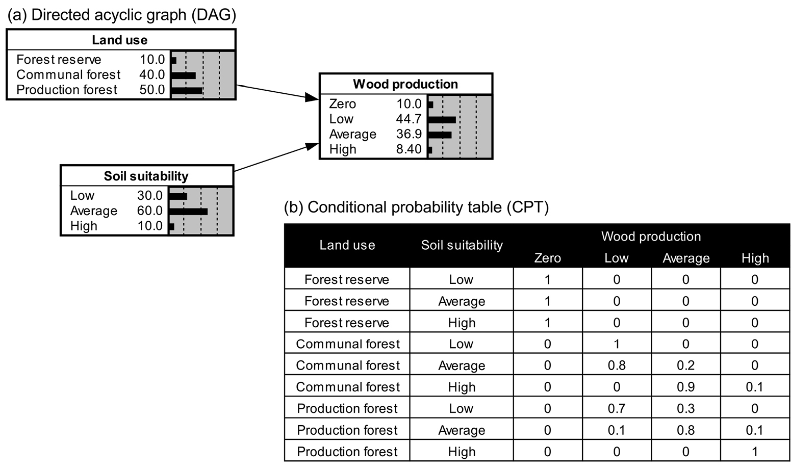
A model example illustrating the structural components of a Bayesian Belief Network: (a) the directed acyclic graph (DAG) and (b) the conditional probability tables (CPT).
The application of BBNs generally consists of inserting new information or evidence in one or more nodes of the model and, subsequently, analysing the resulting belief changes. This new information can be deterministic or probabilistic depending on whether the information implies that a state is exactly known or not. Figure
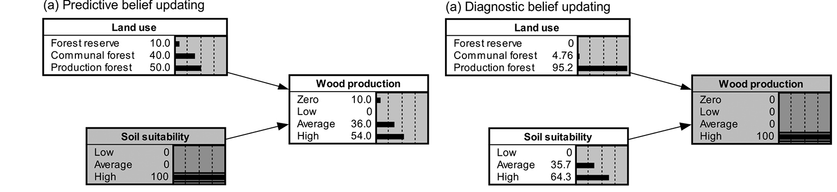
Strengths and weaknesses
Although BBN models have been used since the 1980s, applications were restricted to medical diagnosis, where BBNs were used to combine probabilistic information on disease occurrence with probabilistic information on symptom development to support the process of reaching a diagnosis. Late in the 1990s, BBNs were introduced in the environmental modelling domain, predominantly because of their ability to explicitly account for uncertainty, an important aspect when natural processes are being modelled. A second important reason for their adoption was the potential of the technique to integrate expert knowledge in the modelling process. Expert knowledge can be used to develop the network structure or to populate the model's CPTs with subjective probabilities, which are also referred to as beliefs. This functionality is especially useful in case variables need to be included for which no supporting data are available, a frequently occurring problem in ecosystem service modelling. A final strength of the modelling technique is its graphical nature. Due to this feature, BBNs are transparent models that are relatively easy to grasp. This means that non-expert stakeholders can be involved in model development.
Another important advantage in the context of ecosystem service modelling is that BBNs fit extremely well in the 'ecosystem services cascade' which has been used as a basis for many ecosystem service studies (see Chapter 2.3) (Figure
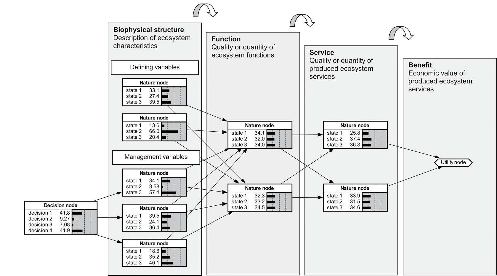
Although a linear representation of the ecosystem service production process might facilitate system understanding, in reality most ecosystem service delivery processes are non-linear and involve a range of feedbacks which BBNs cannot easily take into account. Developing several models for successive time steps of a system and chaining them afterwards is a 'workaround' that mimics feedbacks with BBNs. Such time-sliced models, however, often become very complex and lack transparency. Another important drawback of BBN is the obligation to discretise continuous variables so that they can be represented as having states in a node. To minimise information loss discretisation methods need to be chosen carefully. Nevertheless, for some applications, nodes with discrete states are more easily understood than continuous variables. If discretisation thresholds are chosen in accordance with the aim of the model, discretisation does not necessarily lead to information loss. Where information loss is not acceptable, more complex software packages are available that enable the use of continuous variables in BBNs.
The drawbacks discussed above all suggest that BBNs are less suitable for modelling complicated processes than some other approaches. Thus, for well-studied services, the added value of using BBNs instead of process-based, validated models is low. The real strength of BBNs lies, however, within the integration of well- and poorly-studied services in one integrated model. Such integrated models might deliver additional insights into trade-offs and synergies among services. In addition, their graphical nature can facilitate stakeholder involvement and social learning, two objectives that are difficult to attain using conventional modelling approaches.
Model development guidelines
To determine which variables need to be included in the model, a variety of knowledge sources can be used. Domain experts can be consulted to select variables that are important for biophysical modelling of service provision, while stakeholders can be consulted to include social interests, i.e. the ecosystem services that are considered important in the study area, or the values associated with them. The type of endpoint being modelled is also an important aspect to consider when including ES in the model. These endpoints can be biophysical quantities, scores that represent social values or monetary values of generated benefits. Modelling the full ES cascade, up to the final benefits, can be attained by integrating studies from different research fields such as economics and sociology.
To select input variables, two things need to be considered, namely the management options that need to be evaluated by the model and whether spatial application of the model is desired. For spatial modelling applications, spatial data on the model's input nodes or on their proxies need to be available. To make management evaluation possible, all variables that are influenced through management and that impact ecosystem service delivery need to be included.
Discretisation of continuous variables is the next step in the model development process. In general, the number of states needs to be kept as low as possible. As the number of states directly affects the complexity of the model's CPTs, less effort needs to be invested in CPT quantification in case the number of states is kept low. Thus, a balance needs to be found between reducing model complexity and minimising information loss. Additionally, in case CPTs are learned from data, the number of states needs to be restricted to ensure that sufficient information is available for all state combinations.
To develop the structure of the model, experts are often consulted. To integrate local knowledge in the model structure, stakeholders can also be consulted. As stakeholders and experts are generally not aware of a model's technical restrictions (e.g. the fact that feedback loops cannot be included), modellers need to guide the model development process and, if necessary, adjust the structure afterwards. Although data can be used to create model structures and estimate probabilities using learning algorithms, relations that are defined through this process are not necessarily a result of causality and, therefore, they are sometimes hard to interpret.
Quantification of CPTs is the final step towards implementing the model. A broad range of knowledge sources can be consulted for this, including expert and stakeholder knowledge, empirical equations, simulations with existing models, literature data and field data. Although data might seem the most objective way to quantify a CPT, datasets are often not sufficient to fully quantify a model's CPTs. In these situations, experts can be consulted to define prior CPTs and data can be used to update CPTs; this is a typical Bayesian workflow. Aside from CPT quantification, the probability tables of the input nodes also need to be quantified. If input nodes represent spatial variables, histograms of spatial datasets can be used to populate these probability tables.
To increase the credibility of a Bayesian Belief Network, model validation needs to be performed. To evaluate a model's predictive performance, a broad range of validation metrics are available, similar to those extensively used in other modelling domains. The predictive performance of BBNs, however, is generally low compared to other techniques. While most models only focus on performing one specific task optimally, BBNs try to approximate the joint probability distribution over all variables, mostly at the expense of their predictive performance. Predictive performance is, therefore, generally not the most important aim of a BBN model, especially in the field of ecosystem service modelling. Other evaluation criteria include the ability of the model to describe a system, to enhance social learning and to facilitate decision-making. To evaluate those aspects, evaluation through experts and stakeholders might be more appropriate. The consulted experts and stakeholders for model evaluation are preferably not those consulted during model development.
To perform the above tasks, a range of software packages are available. Frequently used software packages in the ecosystem services modelling domain are 'Netica' and 'Hugin'. They both provide a user-friendly graphical user interface for model development that can potentially be used with stakeholders. Most packages also include algorithms that can be used to train and validate models using existing datasets. Furthermore, through application programming interfaces (API), software packages can be extended with all kinds of tools. Following this approach, BBNs can, for example, be coupled to geographical information systems (GIS). This is an important functionality when BBNs are used for ecosystem service mapping.
Conclusions
As illustrated in this chapter, BBNs have much potential for modelling and mapping ES. They operate at an intermediate level of complexity which makes them especially useful where the volumes of available data and knowledge are not sufficient for empirical or process-based modelling. Additionally, BBNs are useful tools to help structure the available knowledge into comprehensible ways that can support social learning and stakeholder participation in ecosystem service modelling and management studies.
Further reading
- Cain J (2001) Planning improvements in natural resource management. Guidelines for using Bayesian networks to support the planning and management of development programmes in the water sector and beyond. Wallingford: Centre for Ecology and Hydrology.
- Haines-Young R (2011) Exploring ecosystem service issues across diverse knowledge domains using Bayesian Belief Networks. Progress in Physical Geography 35(5): 681-699.
- Landuyt D, Van der Biest K, Broekx S, Staes J, Meire P, Goethals PLM (2015) A GIS plug-in for Bayesian belief networks: Towards a transparent software framework to assess and visualise uncertainties in ecosystem service mapping. Environmental Modelling & Software 71: 30-38.
- Landuyt D, Broekx S, D'hondt R, Engelen G, Aertsens J, Goethals PLM (2013) A review of Bayesian belief networks in ecosystem service modelling. Environmental Modelling & Software 46(0): 1-11.
- Potschin M, Haines-Young R (2016) Defining and measuring ecosystem services. In: Potschin M, Haines-Young R, Fish R, Turner RK (Eds) Routledge Handbook of Ecosystem Services. Routledge, London and New York, 25-44.
Glossary BBN
Node - Graphical representation of the system variables in a Bayesian Belief Network model.
State - A value, discrete class or qualitative level to which a variable can be assigned. Each variable in a Bayesian Belief Network model has a set of states it can manifest.
Probability distribution - The set of probabilities assigned to the states of a variable that express the probability that the variable equals one of its states. This set of probabilities always sums up to 1.
Arrow - Graphical representation of the causal relations amongst the system variables in a Bayesian Belief Network. Each arrow flows from a parent node to a child node.
Conditional probability - The probabilities that quantify the model's causal relations and express the probability distribution of a child node given the status of its parent nodes.
Conditional probability table or CPT - A table that contains probability distributions over a node's states conditional on all possible combinations of its incoming nodes' states.
Directed acyclic graph or DAG - Graphical representation of the system being modelled by means of nodes that represent system variables and arrows that represent causal relations among the system variables.
4.6. Applying expert knowledge for ecosystem services-quantification
Ecosystem services (ES) are a complex field of study. The application in practice poses several additional challenges. Although ES quantifications can built on existing experience, methods and data (see Chapters 4.1-4.5), specific human-environmental system settings, policy frameworks and characteristic ES need to be considered thoroughly. Expert involvement can provide information in cases where other sources are lacking, efficiently generating results and validating maps. Moreover, structural expert involvement in trans-disciplinary projects can improve effectiveness of projects which are geared at real world impact. This chapter provides basic considerations on expert involvement and puts forward some guidelines to tackle challenges related to trans-disciplinary mapping.
Why experts
Expectations towards ES science and application are very high. The global socio-ecological challenges which researchers are aiming to tackle are both urgent and important. Still, the amount of trust and public resources going to ES studies and mapping is relatively high compared to their current impact on solving real world problems.
Applied ecology and sociology are considered complex fields, combining several disciplinary frameworks, ways of thinking and related methods. ES, at the crossroads of applied ecology, economy, sustainability science and social sciences, can be defined as "super-complex". Super-complex or so-called wicked problems require engagement of several theoretical disciplines and practitioners in actual implementation from the very onset of the problem-solving process.
What looks like just a simple ES map is often a complex combination of selected quantitative data, proxies and expert estimates, qualitative judgements, theoretical assumptions, technical choices and communicative visual goals (see Chapters 3.3 and 6.4). The quality of the actual mapping process directly determines the qualities of the map in all its aspects (credibility, relevance, clarity, usefulness; see Chapter 5.4). Creating a map which lives up even to minimal real world application ambitions obliges the involvement of 'experts' to legitimise, clarify, improve and validate maps to be relevant for any specific application context.
What makes an expert
Delineating who is an expert and who is not is not straightforward. From the above, it is clear that, when solving real world problems, merits of diploma and discipline are not enough by far. A bright GIS technician is certainly a required expert, but without complementary input from the ecology expert, the modeller, the economist and the social scientist, there is actually nothing to map or to interpret. Also, without the local or topical experts to put the socio-economic and natural science theories into a specific context, maps will be hard to validate. Moreover, without the expert who connects specific policy demands, cultures and know-how, implementation of the maps into actual solution strategies will rarely happen. And finally, deciding on societal importance of issues or values of specific ES to decide upon trade-offs requires input from policy makers and/or the direct end-users of these services.
All these types of knowledge are indispensable for the mapping process, and not necessarily related to education level or strictly technical skills. The central idea is that all experts - or knowledge-holders - need to be thoughtfully engaged.
Selective expert engagement
From the point of view of a technical mapping project, involving experts is often regarded as costly, tedious and complicated. We will show that structural expert involvement will add value to the whole process of map creation and effective problem-solving. Three examples of selective engagement are discussed here. The section, following this discussion, returns to address the more profound expert engagement of trans-disciplinary research.
1. Experts plaster the holes in your data
The most commonly heard argument for engaging experts is to provide 'educated guesses' and estimates of ES supply, locations or contexts where a given dataset or model is not providing quantitative information. Indeed, this is a highly effective way of filling in missing data to obtain a dataset which allows the creation of a map. The explicit assumption is that these estimates are 'second choice' and 'less reliable', and best replaced by model outputs as soon as these become available. Note that this technical argument disregards the fact that quantitative models (see Chapter 4.4) have originally been compiled and designed by experts. Often they are applied/extrapolated to another context by implementing expert-based modifications and assumptions. In addition, many aspects of ES mapping are simply not quantitative in the natural science sense: economic data, valuations, ecological quality estimates - they are all based to a large extent on qualitative expert estimates. Collaboration among diverse and multiple experts from the onset could help to avoid the disciplinary bias of the experts that happen to steer the mapping process.
2. Experts generate quick results
A second pragmatic reason to involve experts is that they provide quick access to a broad range of knowledge and comparable ES maps can be obtained in a relatively cost-efficient way. Indeed, with a minimum of resources, maps can be obtained, with known reliability and high credibility (provided that some basic rules are followed concerning which experts to select, the representativeness of this selection and how to evaluate expertise levels). A process model-based quantification (tier 3; see Chapter 5.6.1) does not necessarily deliver more useful or 'true' results than a tier 1 (expert-based relative scoring) or a tier 2 quantification. In an optimum case, several approaches (tiers) can be applied for the same ES in one region and the results can be triangulated in order to cross-validate and increase reliability. There is a risk that an overly pragmatic approach ignores existing data and models already available. In addition, involved experts are frequently frustrated when the highly detailed and complex knowledge they hold is reduced, for example, to a comparable scoring format for predefined indicators. Much more potential lies in the combination and comparison of diverse approaches from different mapping tiers (see Chapter 5.6.1) and quantification methods (see Chapters 4.1-4.4), from the start.
3. Experts fix your credibility
A third common application of expert engagement is ensuring the local or topical validity of the maps created. This concerns local ecological knowledge or elicitation of societal values, but it can also entail spatial validation and adaptation of resulting maps. Although the type of validation can vary, this step is essential for any map which is meant to provide reliable and credible input to decision-making.
The difficulty with such methods and related results is that these often do not come in before the end of a study. Experts are confronted with an end-product which is not always part of a clear process or linked to a recognisable problem. Maps represent highly complex and variable data types, combinations and technical choices in a single, static 2D representation (see Chapter 3.2). Apart from assessing the overall plausibility of the result and 'recolouring' local corrections, information to (re)calibrate models or assess credibility of assumptions made is very hard to obtain. Moreover, if a map turns out not to be useful at all, it is often far too late to change course.
A stakeholder analysis, a knowledge-needs inventory and an engagement strategy at the start of an ES mapping project allows the involvement of key experts (including local/topical experts) and guarantee validation and credibility in order to develop an effective map product.
All three selection-perspectives are pragmatic and instrumental to improve quality, efficiency and effectiveness of mapping projects. Still, these perspectives regard the mappers as project owners, mandated to select 'other experts' for a certain purpose and within a restricted window of engagement. In the next section, we show that a trans-disciplinary approach not only combines the advantages mentioned above, but provides additional benefits for the effectiveness of a mapping project.
Structural engagement of experts
Mapping ES in the context of real world problem-solving needs to go further. Structural engagement of experts departs from a different paradigm. The underlying principle is that there is no de facto distinction between experts and laymen, or between stakeholders and researchers. All people involved in, or potentially affected by, the ES mapping project are stakeholders as well as experts in a certain aspect.
Such a trans-disciplinary viewpoint has two immediate consequences: first, the researchers mandated to perform the mapping project depart from a humble attitude (see Chapter 5.4). Second, experts/stakeholders outside of the actual project team are 'promoted' to the level of potentially indispensable knowledge-holders and project-owners. These include people commissioning the project, topical experts on certain ES, technical experts on different methods, experts on local or thematic context into which the mapping project is framed and people actually depending on ES.
The above does not mean, of course, that every mapping project should involve large numbers of experts throughout the project in order to be effective. The actual number of experts is not the issue here, but it is their competence, diversity, qualification and role they have in the project. In the following section, a theoretical illustration of a mapping project's cycle is presented. This example imagines an ideal project without issues of policy restrictions or budgetary constraints.
1. Scoping
This first phase sets out clear project goals, adding requirements and conditions for well-defined final map products as well as concerning inclusion of various viewpoints in the process. A broad and realistic selection of experts is made to join the project team and co-design, conduct, steer and evaluate the mapping project.
Questions to answer:
Why is the project needed? Which problem needs to be solved? Who are the end-users of the maps? What are the maps going to be used for exactly? Who will be affected by the envisioned solution? How dependent are different people/groups on the human-environmental system, how large is the potential impact on their well-being? What power or representation do they have, to what extent can they govern their own environment?
Expertise needed to answer these questions:
- Experts from policy and administration commissioning the project;
- Experts from the end-user side concerning format and requirements of the map (see Chapter 5.4);
- Technical expertise on policy and defining client demand for product development;
- Experts on various stakeholder points of view, directly or by representatives (e.g. NGOs);
- Technical expertise on stakeholder analysis and participation of special groups.
2. Method selection and project design
This phase develops an agreed-upon work plan, project governance structure and workload distribution.
Questions to answer:
What methods and data do we need to create the product? What methods and know-how do we need to set up the process accordingly?
Expertise needed to answer these questions:
- Experts from different disciplinary fields;
- Technical mapping experts;
- Specialist experts on detailed sub-topics (e.g. certain ES, habitats, land use practices, stakeholder groups);
- End-user experts to follow up on map usability;
- Policy experts to follow up on relevance;
- Stakeholder representation to follow up on different goals and conditions;
- Technical expertise to design and facilitate participation and feedback process between product developers, end-users, commissioning bodies and stakeholders.
3. Creating reliable maps
This phase produces maps with transparent reliability, conscious decisions affecting interpretation and best available knowledge, while safeguarding purpose, usability and local/thematic specificities.
Questions to answer:
How can we include and combine various data types? How can we determine reliability of different types of data and knowledge? How can we select data and communicate reliability? How do we make technical choices which impact the outcome (e.g. interpretation of maps)?
Expertise needed to answer these questions:
- All experts and stakeholders need to reach agreement on choices concerning reliability within the particular project;
- Different experts on similar topics need to triangulate and cross-validate methods and results;
Technical experts need to design and facilitate efficient decision processes and communicate decisions.
4. Implementation of the maps
This phase ensures effective implementation of the products as well as adherence to the agreed goals. Ideally, this phase runs throughout the project, in order to test early versions of the maps and adapt methods (or goals) based on these tests.
Questions to answer:
How can we ensure effective application of the maps in the envisaged solution/instrument? How can we evaluate distance to target?
Expertise needed to answer these questions:
- All experts and stakeholders need to agree on engagement in implementation and criteria for evaluation;
- End-user experts need to test application and provide feedback.
Solutions and recommendations
- Clear goals. Being effective requires the right product, produced in the right way. Clearly formulated goals are essential.
- Diversity. The best people should be identified with the diverse skills and knowledge types needed. Consider them equal regardless of their diplomas and promote this attitude.
- Facilitation. Do not think that a trans-disciplinary process will run itself. Project facilitation is a skill, and skilled people will be needed to keep the process running smoothly.
- Parsimony. Do not overdo it. Weigh costs and efforts against stakes. Be pragmatic when needed, but without forsaking the project goals. Adapt unrealistic goals to more realistic objectives.
- Testing and evaluation.
- Do not expect that your team will produce a perfect product at the end of the project. Look for the weaknesses in the project and address them. Test maps as soon as possible and avoid the trap of self-evaluation. The sooner a weakness or failure is identified, the greater chance there will be of finalising your project with a high level of success and impact.
Further reading
- Bradshaw GA, Borchers JG (2000) Uncertainty as information: narrowing the science-policy gap. Conservation Ecology 4(1): 7.
- Cornell S, Berkhout F, Tuinstra W, Tabarae JD, Jager J, Chabay I, de Wit B, Langlais R, Mills D, Moll P, Otto IM, Petersen A, Pohl C, van Kerkhoff L (2013) Opening up knowledge systems for better responses to global environmental change. Environmental Science & Policy 28: 60-70.
- Drescher M, Perera AH, Johnson CJ, Buse LJ, Drew CA, Burgman MA (2013) Toward rigorous use of expert knowledge in ecological research. Ecosphere 4: 1-26.
- Gunderson LH, Holling CS (Eds.)(2002) Panarchy. Island Press, Washington Covelo London.
- Hay I (2010) Qualitative Research Methods in Human Geography. 3rd Edition. Oxford University Press.
- Jacobs S, Burkhard B, Van Daele T, Staes J, Schneiders A (2015) The Matrix Reloaded: A review of expert knowledge use for mapping ecosystem services. Ecological Modelling 295: 21-30.
- Seidl R et al. (2013) Science with society in the anthropocene. Ambio 42(1): 5-12.
- Voinov A, Seppelt R, Reis S, Nabel JEMS, Shokravi S (2014) Values in socio-environmental modelling: persuasion for action or excuse for inaction. Environmental Modelling and Software 53: 207-212.
Chapter 5. Ecosystem services mapping
5.1. What to map
Introduction
Ecosystem services (ES) originated as a concept that reflects the value of nature for humans and provides additional reasons for protection and sustainable management of ecosystems (see Chapter 2.3). Many ES face spatially explicit pressures or rely on anthropogenic contributions such as technology, energy or knowledge. ES maps can help to uncover risks for ecosystem health, unsustainable use of potentials to provide a service, harmful impacts on a landscape, impaired spatial flows of ES as well as mismatches between ES supply and demand (see Chapter 5.2). Such information can indicate where to improve ES provision and where to prioritise nature and biodiversity conservation.
Multiple components play a role in ES provision and use which can be mapped, assessed and monitored. ES can be mapped and assessed using quantitative indicators or qualitative estimations. ES mapping and assessment include ecosystem properties and conditions, ES potential, ES supply, ES flow and ES demand which we generically define in the next sections.
ES mapping terms and their relationships
The framework presented here aims to depict different aspects of ES important for mapping. Our framework bridges variously interconnected ecosystems and socio-economic systems, including the interactions between their components. Figure
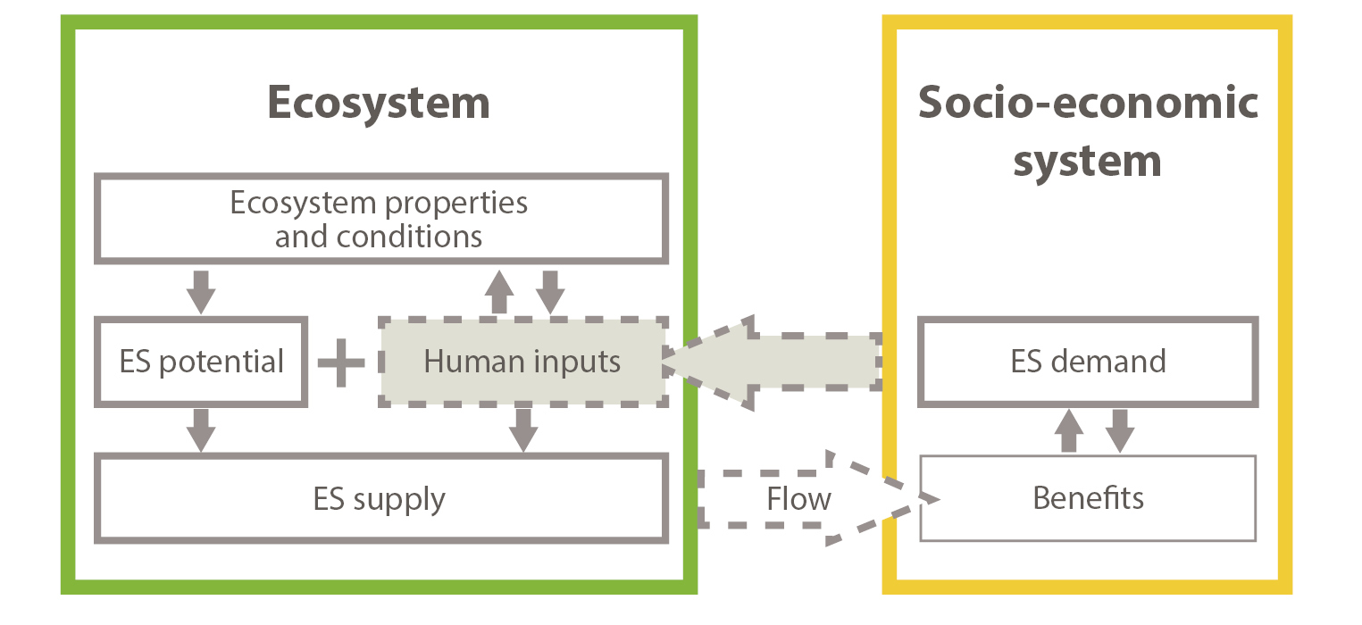
Mapping aspects of ES (own illustration, adapted version of the the ES cascade by Haines-Young & Potschin (see Chapter 2.3),
Ecosystem properties and conditions provide the ecological basis for ES potentials which, together with human inputs, form a capacity of a social-ecological system to provide ES (ES supply). ES flows (i.e. the actual use of ES) can be a fraction of this supply, or be higher in case stocks are depleted or ecosystems are unsustainably used. Demand for ES steers ES flows, i.e. without a demand for a service, there is no actual use. This demand can, however, be higher than actual flow, for example, in cases where societal preferences for specific services remain unsatisfied. Within the socio-economic system, benefits arise from several kinds of ES use depending on the demands of concerned people. Feedbacks from the socio-economic system such as land use change, landscape maintenance or environmental pressures, affect the ecosystem and thereby the ES supply. The following sections explain these terms in detail.
Ecosystem properties and conditions
Definition: Properties describe the character, structure and processes of an ecosystem. Conditions refer to the integrity and health status of an ecosystem which determine its ability to generate ES (see Chapter 3.5). Land use or land cover provide the basis of many ES maps. Beyond that, ecosystem properties such as soil type, slope gradient and inclination, climate conditions and the position in relation to a shoreline or within a watershed are properties that essentially control the supply of many ES. Features of landscape structure like density of certain objects, edge conditions, connection and shape of areas can also be very important. Ecosystem conditions, however, comprise much more: for instance, the load of pollutants, species composition and health may be crucial preconditions for ES.
Delimitation: Properties and condition reflect both the natural ecosystem state and the type of ecosystem as result of a specific land use. Since the condition for ES supply differs between specific ES, the scope of related assessments has to be defined very carefully per ES.
Necessity and applicability: Indicators for ecosystem properties and conditions should be applied to different protection goods or land use classes. They are relevant because they provide the spatial and physical preconditions for ES (see Chapter 2.2). ES potentials can, for example, give a reference point for planning and scenarios (see Chapter 7.2). Both the individual patches' land use and land cover and the configuration and arrangement of such patches, are important for ES supply. Therefore, the landscape structure with its mosaic of patches should be considered (see Chapter 5.2).
Possible indicators: Land cover can provide an essential database for ES mapping. The CORINE land cover dataset is often used in European studies (see Chapter 3.5). At national level, land use data from land survey or habitat mapping often are available. Additional data need to be integrated in more detailed evaluations (see Example 1).
Large contiguous areas of woodland are vital for nature protection by offering habitats for animals and plants and provide people with areas for relaxation. The size of uninterrupted woodland, not dissected by roads and railways, is an important criterion for ecosystem conditions.
Ecotones are transitional areas between habitats. As such, they are home to a particularly rich variety of species, not only those of the adjacent communities but also species that have become specialised to the ecotone itself. In open landscapes, such elements are important as habitat for pollinating insects and for other beneficial organisms. At the same time, a landscape with high proportions of such elements is very attractive for human recreation. In this context, landscape configuration with ecotones is an indicator for ecosystem condition. The calculation of the perimeter of forest-dominated ecotones takes account of all hedges, tree rows and the margins of small copses as well as all forest margins (see
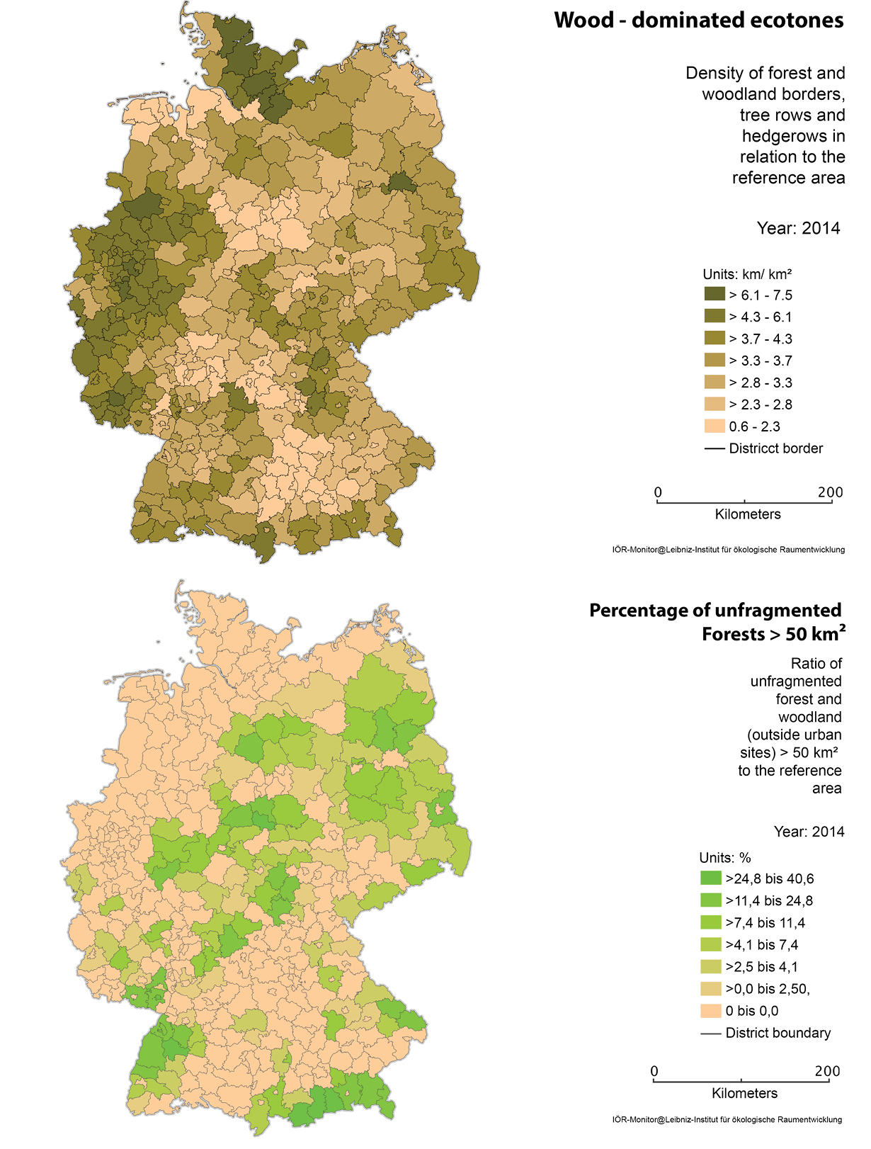
To indicate the gross potential of crop production, the Natural Yield Potential from the Soil Atlas of Saxony, Germany was used. Comparable maps are available for most countries of the world. In a two-stage procedure, first the soil fertility was assessed using field capacity, capillary moisture, cation-exchange capacity and base saturation. Second, the ratio of actual vs. potential evaporation, the length of the vegetation period and slope gradient were taken into account, resulting in five degrees in total. Technical measures such as fertilisation, liming, plant protection and irrigation were excluded here (see
Ecosystem properties and conditions are directly linked to the state of biodiversity. A high level of biodiversity - in most cases - underpins the supply of multiple ES (see Chapter 2.2).
ES potential
Definition: ES potential describes the natural contributions to ES generation. ES capacity is often used synonymously. ES potential measures the amount of ES that can be provided or used in a sustainable way in a certain region given current land use and ecosystem properties and conditions. It is recommended to regard this potential for a sufficiently long time period.
Delimitation: The (natural) ES potential is often supplemented by human system inputs to generate ES supply (see Section Human inputs). The actual provision (co-production) of ES (flow) sometimes includes large human efforts, is strongly dependent on technological refinement and can be very difficult to determine.
Necessity and applicability: In terms of ES potential, the ecological carrying capacity and resilience need to be considered. ES potential allows the distinction between a realised ES and the opportunities and limits of use which is often meaningful for planning purposes, scenarios and management issues. Sometimes, an indicator for ES potential can help to better understand and calculate physical indicators for regulating ES supply.
Possible indicators are, for example, the Muencheberg Soil Quality Rating (SQR), metrics for relief diversity and the share of water bodies as part of landscape aesthetics as well as proxies for processes such as groundwater recharge rates.
ES potential is particularly applicable for planning, management and predictive research purposes. Since it is conceptualised hypothetically and for the long term, ES potential should not be assessed for short time periods (such as for only one season). Preferably, ES potential should be orientated on natural regeneration rates. Direct human interventions such as fertilisation, technical energy inputs or breeding and genetic engineering should not be considered as contribution to ES potentials. In contrast, land use type (grassland, field, forest, settlement) and the consequences of long-lasting or very strong impacts such as mining have to be considered naturally. A distinction of a real 'natural' state that contributes to ES is not straightforward.
ES supply
Definition: Supply is the provision of a service by a particular ecosystem, irrespective of its actual use. It can be determined for a specified period of time (such as a year) in the present, past, or future.
Delimitation: The amount of ES supply depends on natural conditions and often on human inputs (see below), such as land management contributions, knowledge and technology. Though there are some ES without human co-production, they may nevertheless depend on ecosystem preservation. ES supply also includes stocks of natural assets as starting points of the flows of material, energy, information and organisms as results of both ecosystem potential and human co-production.
Necessity and applicability: ES supply is a central subject to be mapped and can be considered a complement to ES demand (see below).
Possible indicators are average yields of crops, wood regrowth in forests, flood retention in catchments or floodplains, amount of carbon stored in soil and vegetation, relative reduction of noise or pollutants, aesthetics of scenery.
ES flow
Definition: Flow is a measure for the amount of ES that are actually mobilised in a specific area and time. Driven by a demand for a service, ES supply is turned into ES flows (Figure
Forest stocks and wood growth are recorded by a forest inventory every 10 years in Germany. Wood regrowth as supply indicator results in 122 million m? per year (comparable to a logging of 84 million m? in 2013). It describes only the status quo; another wood re-growth could be realised at different stock levels, for example, by changing the tree species and age structures = "managed potential". The wood stock in German forests, which may also be regarded as supply, is 3.7 billion m?, or 336 m? ha-1. But since nobody could use them all, this number gives no meaningful indication (
Flood regulating ES provide excellent examples for linkages of SPAs and SBAs via SCAs. Unlike many provisioning ES, flood regulating ES cannot be supplied and imported from remote areas. SPAs and SBAs need to be physically connected (e.g. by a water body or stream) or located in the same process unit (e.g. a watershed). The "flow" of flood regulating ES takes place by spatial units that are able to capture excess water (e.g. from torrential rain) and to regulate the surface water runoff contributing to floods. Humans and their properties benefit from this regulating ES flow by lower amounts of floodwater reaching the SBA. The ES demand exceeds the supply in case of flood hazards. Land use change (e.g. afforestation) in the SPAs can help to increase flood regulating ES flows (see
Delimitation: Service flow can be constrained by an inadequate ES supply which would lead to exceedance of the ES potential. This again may lead to an overuse of given ES potentials, degradation of natural capital or to unmet ES demand.
Necessity and applicability: ES flow maps can unfold spatial mismatches between ES providers and beneficiaries. If there are essential natural processes supporting these interactions between providers and beneficiaries, ES flow mapping gives insights to Service Connecting Areas (SCA; see Chapter 5.2). Their conditions such as possible barriers or other features shaping the flow are items that can be mapped meaningfully.
Possible indicators are fish catch, timber logging, bioenergy gain, groundwater extraction (by wells), flood peak reduction, visitor numbers.
ES flow should particularly be included in integrative supply-demand assessments. There is a broad range of process models (see Chapter 4.4), expert knowledge (see Chapter 4.6) or monetary valuation methods (see Chapter 4.3) which can be applied here.
ES demand
Definition: Demand is the need for specific ES by society, particular stakeholder groups or individuals. It depends on several factors such as culturally-dependent desires and needs, availability of alternatives, or means to fulfil these needs. It also covers preferences for specific attributes of a service and relates to risk awareness. Demand links ES to particular beneficiaries. This means that without a demand for a service, there is no flow. Beneficiaries express demand and can have the power to translate this demand into an actual ES use. Demands for some ES (such as several regulating ES) might be uncovered, or certain groups of society might be unaware that they actually benefit from an ES.
Delimitation: Demand can be different from flow which measures the actual extraction of a service within a region. Demand can, for example, be higher than flow within that particular region. This means, when demand is realised, it could be fulfilled through services that come from another region. For instance, many provisioning ES (e.g. food, timber, energy) can be imported. The demand for carbon sequestration (ES climate regulation) can be fulfilled by a region with a high potential to sequester carbon or cultural ES such as recreation can be actively used in another region through travel (see Chapter 6.2). The phenomenon of regionally-unmet demand is common to many ES and so far we have only started to understand the long-distance effects between different regions caused by inter-regional ES use. (Regional) demand could also be lower than flow, in case ES are exported. Demand is then expressed by other social-ecological systems while ES flow takes place in the region of interest.
Using amongst others, travel costs, presence of viewpoints, distance to forest and coast, population and income statistics,
Necessity and applicability: Demand can change over time and can show an uneven pattern across space. As a result, it makes sense to map demand independently from potential, supply and flow. Regional demand can exceed the (regional) supply considerably and, through an increased flow, this could result in unsustainable regional levels of extraction or use of a service so that flow could exceed ES potential. As a consequence, local ecosystems are at risk of overuse or ecosystems in other parts of the world are degraded by land use change (ES footprint).
Possible indicators are vulnerability of people or value of endangered assets for flood risk, desirable attributes for recreation, accessibility and travel costs of visitors, socio-economic valuation and stakeholder perceptions.
Demand involves human preferences which can be determined through questionnaires, but also involves basic needs (e.g. unpolluted air) and actually used ES (e.g. flood protection at a riverside) even when people are not aware of them. Aspects of risk aversion can be based on assumptions, be modelled or by enquiries (stated preferences). In the case of provisioning ES, the beneficiary could be a farmer who benefits from an intact agricultural ecosystem. It could, however, also be the regional population that formulates the demand for locally-produced food.
Human inputs
Definition: Human inputs encompass all anthropogenic contributions to ES generation such as land use and management (including system inputs such as energy, water, fertiliser, pesticides, labour, technology, knowledge), human pressures on the system (e.g. eutrophication, biodiversity loss) and protection measures that modify ecosystems and ES supply.
Delimitation: Human inputs often emerge as harmful impacts to ecosystems caused by monocultural land use, land use change or intensification. Today, most ecosystems and the services they provide are used and influenced by humans.
Necessity and applicability: Humans perform multiple roles in ecosystems acting as managers, but also as co-producers, distributors or beneficiaries of ES.
Possible indicators are land use type and intensity, load of pollutants, material or energy input (such as nitrogen), effort of landscape maintenance, further contributions to ES.
Human impacts are accompanied in many cases by substantial losses of biodiversity.
Particular attention should be paid to human inputs since they may alter ES supply considerably and this impact differs spatially. Not only targeted land use activities influence the integrity of ecosystems, but also the utilisation and improvement of ES can impact other services as well. Resulting ES trade-offs (see Chapter 5.7) are important to review, but are often hard to map.
The indicator Gross Nitrogen Surplus (GNS) indicates the potential surplus of nitrogen (N) on agricultural land. For EU-27, it remained relatively stable between 2005 and 2008 with about 51 kg N/ha/year. The GNS for the EU-15 reduced between 2001 and 2008 from 66 to 58 kg N/ha/year. The GNS was highest between 2005 and 2008 in countries in the North-West of Europe (Belgium, the Netherlands, Norway, UK, Germany, Denmark) and the Mediterranean islands Malta and Cyprus, while many of the Mediterranean (Portugal, Italy, Spain, Greece), Central and East European countries show the lowest N surpluses (Eurostat).
Conclusions and recommendations
Depending on the scope of application, ES maps can show different contextual aspects of ES which are spatially heterogeneous in a different way and therefore relevant for ES mapping. Depending on data availability and the policy question or information needs at hand, mapping of one or two of these aspects might be sufficient. It is recommended to map only such aspects that can be derived from reliable data. When monitoring or systematic balance over time is requested, data and indicators have to be double-checked for comparability which can also depend on methods or technology of data collection and on appropriate indicator selection.
Further reading
- Ala-Hulkko T, Kotavaara O, Alahuhta J, Helle P, Hjort J (2016) Introducing accessibility analysis in mapping cultural ecosystem services. Ecological Indicators 66: 416-427.
- Albert C, Galler C. Hermes J, Neuendorf F, von Haaren C, Lovett A (2015) Applying ecosystem services indicators in landscape planning and management: The ES-in-Planning framework. Ecological Indicators 61, Part 1: 100-113.
- Bastian O, Syrbe R-U, Rosenberg M, Rahe D, Grunewald K (2013) The five pillar EPPS framework for quantifying, mapping and managing ecosystem services. Ecosystem Services 4: 15-24.
- Burkhard B, Kandziora M, Hou Y, Muller F (2014) Ecosystem service potentials, flows and demand - concepts for spatial localisation, indication and quantification. Landscape Online 34: 1-32.
- Fischer A, Eastwood A (2016) Coproduction of ecosystem services as human-nature Interactions - An analytical framework. Land Use Policy 52: 41-50.
- Grunewald K, Herold H, Marzelli S, Meinel G, Syrbe R-U, Walz U (2016) Assessment of ecosystem services at the national level in Germany - illustration of the concept and the development of indicators by way of the example wood provision. Ecological Indicators 70: 181-195.
- Jones L, Norton Z, Austin AL, Browne D, Donovan BA, Emmett ZJ, Grabowski DC, Howard JPG, Jones JO, Kenter W, Manley C, Morris DA, Robinson C, Short GM, Siriwardena CJ, Stevens J, Storkey RD, Waters G, Willis F (2016) Stocks and flows of natural and human-derived capital in ecosystem services. Land Use Policy 52: 151-162.
- Liu J, Yang W, Li S (2016) Framing ecosystem services in the telecoupled Anthropocene. Frontiers in Ecology and the Environment 14: 27-36.
- Nedkov S, Burkhard B (2012) Flood regulating ecosystem services - Mapping supply and demand, in the Etropole municipality, Bulgaria. Ecological Indicators 21: 67-79.
- Remme RP, Edens B, Schroter M, Hein L (2015) Monetary accounting of ecosystem services: A test case for Limburg province, the Netherlands. Ecological Economics 112: 116-128.
- Termansen M, McClean CJ, Jensen FS (2013) Modelling and mapping spatial heterogeneity in forest recreation services. Ecological Economics 92: 48-57.
- Villamagna AM, Angermeier PL, Bennet EM (2013) Capacity, pressure, demand, and flow: A conceptual framework for analyzing ecosystem service provision and delivery. Ecological Complexity 15: 114-121.
- Walz U (2015) Indicators to monitor the structural diversity of landscapes. Ecological Modelling 295(1): 88-106.
- Wolff S, Schulp CJE, Verburg PH (2015) Mapping ecosystem services demand: a review of current research and future perspectives. Ecological Indicators 55: 159-171.
5.2. Where to map
The spatial-structural approach
It is an important feature of natural and cultivated ecosystems that they are not evenly distributed across landscapes, coastal or marine areas and they also vary over time. Ecosystem services (ES) are usually generated by ecological processes within their area of influence such as catchments, habitats, natural regions or land use units. This suggests the need for site-specific assessments. Therefore, each ecosystem service should not only be assessed through considering underlying ecosystem types but also with respect to:
- underlying natural regional conditions (geology, landform configuration, soil, climate, etc.),
- its positional relations to main types of landscape (urban, agrarian, near-nature),
- the configuration (landscape structure) of the corresponding units (catchments, natural regions, etc.) with natural resources or land uses,
- the relations between the ecosystem providers of a service and groups of people who make use of it (i.e. beneficiaries) and
- the use, management and maintenance of the respective ecosystem.
Spatial relationships, area types
The holistic approach presented here presumes that complex ecological systems underlie the production of most ES, which can be envisioned as SPUs, or Service Providing Units. For mapping purposes, such an SPU should be regarded as a spatial unit. This opens the way for applying landscape-scale geographic assessment methods based on landscape units corresponding to the area of influence (see above).
In order to avoid terminological confusion with different SPU variants, we term the spatially defined complexes as Service Providing Areas (SPA) (see Text Box 1). SPAs are a promising basis for an inclusive approach of ES at the landscape scale.
Service Providing Area (SPA): spatial unit within which an ecosystem service is provided. This area can include animal and plant populations, abiotic components as well as human actors.
Service Benefiting Area (SBA): spatial unit to which an ecosystem service flow is delivered to beneficiaries. SBAs spatially delineate groups of people who knowingly or unknowingly benefit from the ecosystem service of interest.
Service Connecting Area (SCA): connecting space between non-adjacent ecosystem service-providing and service-benefiting areas. The properties of the connecting space influence the transfer of the benefit (also refer to Text Box 2).
As the service providing areas defined above include entire ecosystems, their constituent populations and underlying biophysical characteristics, the best way of capturing them spatially is as ecological spatial units (e.g. living spaces, water bodies or soil areas) or as area of influence of the respective processes (e.g. catchment areas, flood plains). From this point of view, such biophysically-delineated areas are more suitable for analysis than administrative units.
In the spatial analysis framework, however, not only the SPAs are of interest, but also the regions to which their benefits accrue. For example, one might ask: where is the benefit of a given ecosystem service needed? In addition to the service providing areas (SPAs), Service Benefiting Areas (SBAs) should thus be defined in which beneficiaries receive the service (see Text Box 1). In a spatial framework, urban areas, rural settlement areas and especially administrative units could be considered as SBAs. Factors such as population density, social facilities (e.g. schools, hospitals but also parks for recreation) and built structures (residential, commerce or industry buildings) or the number and size of the households, are important as indicators (e.g. per household measures of demand for specific ES).
The service providing and service benefiting areas may overlap, but significant spatial differences are also possible (see example in Text Box 2). If the service providing and service benefiting areas are not adjacent, the properties of the connecting space can have an influence on the provision of the service (see Text Box 2). We include such an interstitial space between service providing and service benefiting areas in our considerations under the term Service Connecting Area (SCA) (cf. Fig.
The floodwater regulation service mainly depends on the character of the watershed that is upstream of beneficiaries, whereas the benefit from the reduced flood risk in the populous cities along the flood plains is presumably highest in the more built-up lower reaches. This raises the question of whether the residents at the upper reaches should unilaterally forego development options in favour of the downstream riparian beneficiaries and, if so, how much compensation should they be entitled to? Should the most vulnerable houses in a downstream settlement be resettled out from the flood plains or protected better? The service connecting area also plays an important role, since, for example, the channel geometry, tributary streams, natural floodplains and wetlands and reservoirs or other grey infrastructure can strongly modify the severity of a potential flood.
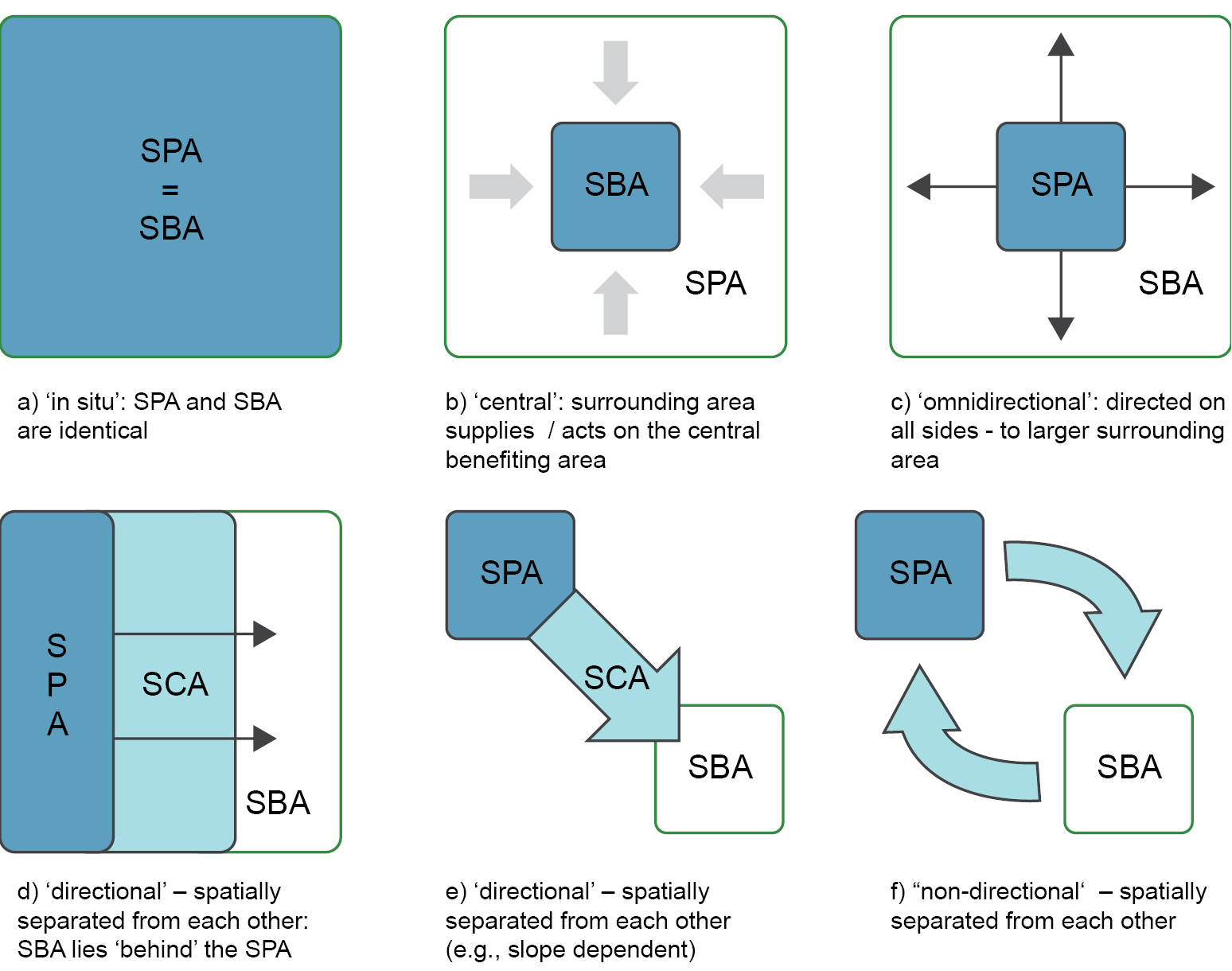
Types of spatial relations of Service Providing Areas (SPA), Service Benefiting Areas (SBA) and Service Connecting Areas (SCA) (adapted and extended from
The following fundamental types of relations between the service providing and the service benefiting areas can be distinguished (Fig.
- 'in situ': the two area types are identical, i.e. the ES are supplied and in demand in the same area (e.g. the population uses the groundwater of its settlement area),
- 'central demand': the surrounding area provides for / impacts on a central demand area (e.g. a settlement benefits from supply of fresh and cold air which is generated by open spaces in the surrounding),
- 'omni-directional': the service benefiting area surrounds a service providing area independent of direction (e.g., farmland benefits from hedges as a living space for beneficial insects),
- 'directional without dependency on a slope': the service benefiting area is situated "behind" the service providing area, protected as it were with respect to the predominant impact direction (e.g. a residential area protected against traffic noise by a forest),
- 'directional downslope': the service benefiting area is situated downhill (downriver) from the service providing area, i.e. the service is dependent on gravitational processes (e.g. cold air, water, avalanches) and
- 'spatially separated': e.g. drinking water, food production, recreational areas. There can be different connective methods, e.g. natural hydrologic flow within watersheds, infrastructure (pipes/aqueducts) or road/trail networks.
The relation types d, e and f can especially exhibit considerable service connecting areas.
Analysing the spatial structures
Once SPAs, SBAs and SCAs are defined for each ecosystem service (see Table
Examples for Ecosystem Services, which depend on lateral or vertical landscape processes, with associated Service Providing Areas (SPA), Service Benefiting Areas (SBA), Service Connecting Areas (SCA) (adapted from
| Ecosystem Services * | Service providing area (SPA) | Service connecting area (SCA) | Service benefiting area (SBA) |
| P groundwater recharge | Arable land, wood, grassland, wetlands and other open land in a groundwater basin | Groundwater flow paths (with possible contaminated sites and risk areas for the protection of groundwater) | Settlement areas, irrigated areas |
| P drinking water | Headwaters and catchment areas | Bodies of groundwater, streams, rivers, (pipelines); (see Chapter 6.2) | Settlement areas, industry (for production, less for cooling) |
| P fodder for grazing animals | Grassland and forage crops | Pastoral paths | Farms |
| R protection against snowdrift, storm | Forest, road trees, shrubs, hedges | Embankments at roads and railway lines | E.g. roads, railway lines and runways |
| R erosion prevention - by wind - by water | Forest, hedges, bushes, trees and shrubs (grassland, permanent crops) | Field edges, gullies | Areas under cultivation, water reservoirs |
| R flood prevention | Forest, ponds, wetlands, etc. in flood generation areas | Floodplains above benefiting areas | Built-up area in the floodplain |
| R local climate regulation (cold/fresh air) | Open land, parks above cities | Slopes (with or without obstacles) around a city | City in valley |
| R noise reduction | Roadside greenery, wood, ramparts | Areas (if appropriate buildings) around the source of noise | Residential and recreational area |
| R avalanche and landslide prevention | Forest above residential or recreational areas | Slope area | Residential or recreational areas below steep slopes |
| R pollination | Nesting habitats of insects | Radius of flight and foraging habitat | Farms with crops requiring pollination |
| R pest control | Nesting habitats of predators | Foraging habitat | Crop land |
| R stream water purification | Surface water bodies, wetlands | Water catchments | Residential or recreational areas |
| C appreciated scenery | Viewsheds (areas which can be seen from a particular site) | Line of sight, open country | Settlements and touristic infrastructure |
| C recreation activities | Surface water bodies, mountains, wood | Road and path network between SPA and SBA | Touristic lodging units |
- a site characterisation and classification of the potential for providing the service with respect to the required natural processes and their dynamics,
- an analysis of the human usage patterns also regarding their internal structure, for example, through landscape metrics and
- the consideration of the conditions regarding location and neighbourhood according to the respective processes.
The comparison and the positional relations of the service-providing areas to the associated service-benefiting and service-connecting areas form another focal point of the spatial investigation. The characteristics of the service-providing areas are primarily founded on the natural sciences, since they relate to the beneficial natural resources and - if applicable - to those processes which ensure their regeneration. Furthermore, the analysis needs to examine whether investments (protection or management measures) are necessary in order to preserve the service supply capacity. If so, the kind and frequency of the maintenance measures should be determined and the necessary cultivation rules should be known. If the natural capital is reducible (by consumption), the natural capacity to regenerate has to be determined in order to adapt the consumption to the regeneration rate if a sustainable resource management is to be achieved.
The characterisation of the service-benefiting areas also includes further analysis from the social sciences. Especially, users' demands have also to be incorporated into analysis of SBAs. Depending on the area of investigation, the demands, preferences and values of the benefiting population groups represent indicators for the demand for the ES. The size of a population group is an important basis for determining and assessing the service. However, whether threshold values should or must be defined is also crucial for the assessment. This can be the case, for example, with respect to people endangered by natural disasters (e.g. restriction of construction areas because of flood hazards) or to unsustainable resource harvest rates (see above). Moreover, limited or widely demanded resources require clear rules for accessing them in order to avoid "free-rider effects" (benefiting from a service without contributing to it) and misinvestments. The type of access (private, common or public) to a resource and the possibility of excluding people from such access determine the marketability or non-marketability of the ES.
Even if a service connecting area does not exist separately because service-providing and service-benefiting areas overlap, an analysis of the connection properties is useful, since horizontal transfer processes are influenced by landscape characteristics. If there is an interstitial space between the service-providing and the service-benefiting area, this connecting space first needs to be determined more closely, which can at times be difficult. This can be modelled for example using the transport and transformation paths of substances, energy, biota and possibly also information.
Spatial units as the basis of ecosystem services assessments
Depending on the type of the ecosystem service that is being assessed, very different spatial units can be considered for service providing, benefiting and connecting areas (Table
Example for the suitability of landscape units for designation of provision, benefiting and connecting areas.
| Nature and origin of the service | Spatial unit |
| Generated by specific species | Suitable habitats |
| Based on biophysical resources | Natural regions |
| Depending on specific landscape mosaic | Spatial unit with comparable spatial features |
| Generated by an abiotic process | Area of influence of this process |
| Dependent on specific land management practices | Management units |
| Rooted in history and culture | Units of the historic cultural landscape |
| Hydrologic services | Water catchment areas |
| Demand for ecosystem services by people | Administrative units |
- Examples of different types of spatial units for capturing and assessing individual ecosystem services are:
- Single surfaces (patches), landscape elements such as arable field sections or forests provide the spatial basis of reference most frequently used for the overall assessment.
- Administrative units are useful if data are analysed which have such units as a reference basis, such as socio-economic data or legal framework conditions.
- Water catchment areas are typical morphological units which can be delimited well using GIS on the basis of a digital elevation model (see Chapter 3.4). They therefore represent the common reference units for hydrologic services.
- Natural units should be drawn upon if natural properties such as soil conditions, surface forms, climate, geology or vegetation mainly determine a service.
- Landscape units, delimited not only according to natural conditions but also according to land use, are usable for most services, especially for site-scale assessment of ES. These units serve as a reference basis for assessing different aspects of diversity, for determining the spatial heterogeneity and as a spatial framework for practical management.
Conclusions
A decided advantage of a spatial-structural approach is that it makes it possible to understand ES beneficiaries and flows. As soon as it is possible to determine the beneficiary of a service, the benefit of such a service can also be identified. This especially applies when the provision and the use of such services do not spatially overlap. Only this knowledge makes it possible to design incentive systems and fair payment for the providers when they deliver this service (see Chapters 7.2 and 7.3). This is also the prerequisite for ES' availability in the long term.
Further Reading
- Bagstad KJ, Villa F, Batker D, Harrison-Cox J, Voigt B, Johnson GW (2014) From theoretical to actual ecosystem services: Mapping beneficiaries and spatial flows in ecosystem service assessments. Ecology and Society 19(2): 64.
- Bastian O, Grunewald K, Syrbe RU (2012) Space and time aspects of ecosystem services, using the example of the EU Water Framework Directive. International Journal of Biodiversity Science, Ecosystem Services & Management: 1-12.
- Burkhard B, Kandziora M, Hou Y, Muller F (2014) Ecosystem Service Potentials, Flows and Demands - Concepts for Spatial Localisation, Indication and Quantification. Landscape online 34: 1-32.
- Fisher B, Turner RK, Morling P (2009) Defining and classifying ecosystem services for decision making. Ecological Economics 68(3): 643-653.
- Grunewald K, Bastian O (Eds) (2015) Ecosystem Services. Concept, Methods and Case Studies. Berlin, 312 pp.
- Syrbe RU, Walz U (2012) Spatial indicators for the assessment of ecosystem services: Providing, benefiting and connecting areas and landscape metrics. Ecological Indicators 21: 80-88.
5.3. When to map
Setting the scene
Mapping ecosystem services (ES) is often seen as a static three-dimensional problem where space (x, y) and the value of a given ecosystem service (z) are referred as the main factors of analysis. A wide group of examples that follow this approach populate current scientific papers, books and technical reports. The issue with these assessments is that they often consider that the value of a given ecosystem service in a particular place is (a) stable in time or (b) it already encapsulates the effects of the underlying ecological processes/cycles.
Under a spatial notation (x, y, z), ecosystem service supply is represented by a magnitude, a spatial distribution or configuration and an extent. Although perceptive, this approach does not consider that specific ES are often supplied in different moments in time (e.g. pollination, food production and flood regulation) and generate benefits that can be equally temporally displaced (e.g. in flood regulation there is a lag of time between the accumulated decrease of runoff [superficial water flow] by percolation and the actual reduction of the downstream flood plain). This results from the fact that ecological processes/cycles vary through time and, because most ES (namely, production and regulating services) depend on specific ecological processes/cycles, ecosystem service supply is also dynamic. These dynamics can be illustrated by focussing on a specific ecosystem service provider, e.g. a deciduous tree (Figure
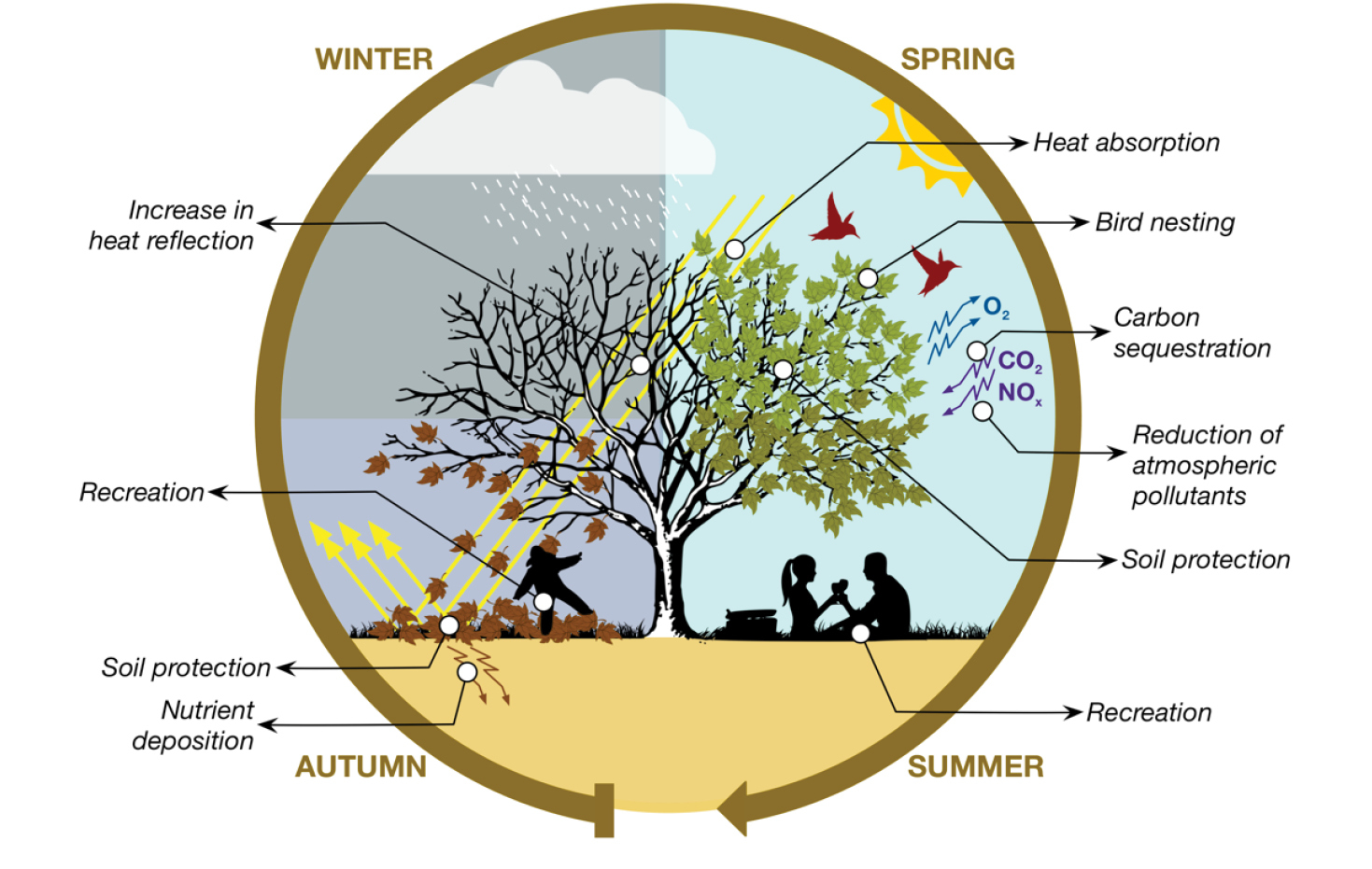
Example of a within-year ecosystem service supply cycle considering a deciduous tree as the focus of ecosystem service supply.
From January to December, the life cycle of a deciduous tree allows for the supply of a relatively large number of ES. Starting in spring, this single tree represents an important support for bird nesting contributing to habitat quality while, at the same time through photosynthetic processes, it captures carbon and other atmospheric pollutants, thus improving local air quality. As time passes, it gives shade for picnics in the summer but it also promotes heat absorption and reduces the albedo effect which helps to reduce heat waves in cities or the probability of fires in forests. At the end of the summer, rain season starts and the same tree contributes to control soil erosion by reducing the erosivity power of precipitation. In the autumn, the leaves fall contributing to local soil fertility. The landscape changes to autumn colours which inspire poets, painters and mountaineers. When winter arrives, the same tree that in summer absorbed heat, now lets the solar radiation pass and thus improves local heat regulation. When isolated, this deciduous tree has a rather narrow potential to supply all of these ES but, when part of a community (e.g. integrated in a deciduous forest), this potential is multiplied and new ES can emerge.
This example serves to show the dynamics and complementarity of ecosystem service supply through time. It also highlights the need to include temporal variations in the assessment of ES, as the likelihood of misrepresenting ecosystem service supply in static assessments is considerable. In fact, time dependency of ES correspond to a very broad and complex issue that includes various time scales, ranging from very short timescales (within a day or a year) to several years, decades or centuries depending on the ecosystem service under assessment. Properly selecting the scale of assessment is fundamental and it mainly depends on the objectives of the assessment and the ecological cycle/process under study. For example, in flood protection, it is possible to focus on hourly variations (if a peak flood is considered and the capacity of vegetation to reduce runoff velocity is studied), monthly variations (if the purpose is to identify hotspots of ecosystem service supply), or yearly variations which can be projected through centuries (if the purpose is to study probability of flood events or projection of trends).
Another dimension of complexity is also the significant mismatch between the potential for ecosystem service supply and the actual ecosystem service supply. This mismatch is also linked to temporal issues.
Consider soil protection as a regulating ecosystem service. In this context, vegetation cover protects soils from being eroded. If vegetation is removed, for instance by harvesting crops, there is an enhanced erosion risk. If we evaluate the temporal dynamics of vegetation cover (here representing the potential to supply soil erosion prevention) and the actual ecosystem service supply (avoided erosion), these variables have two very different temporal distributions resulting in a supply and demand mismatch.
As for the ecosystem service supply, the demand for ES is also dynamic. It usually correlates with the cycles of environmental impact (in the case of regulating services), production cycles (e.g. the requirement for pollination services according to crop cycles), specific consumer demands (e.g. the increase in codfish or turkey demand during the Christmas period), recreation cycles (e.g. the increase in the demand for hiking areas during the summer time), amongst others. The potential differences between the dynamics of demand and supply of ES are among the drivers for over-exploitation of ecosystems making the evaluation of temporal dynamics even more significant.
Ecosystem service dynamics
Assessing ecosystem service potential, supply and demand (see Chapter 5.1) requires a thorough understanding of ecological cycles and ecosystem service mechanisms. Both of these are dynamic and entail the recognition that an ecosystem service is dependent on multiple simultaneously occurring processes with different (often competing) objectives and that ecosystem service supply is secured by different ecosystem service providers with their own specific ecological cycles, targets and trends.
This recognition is critical when assessing ecosystem service supply but it also depends on the objectives of the assessment and on the research question that is being addressed. Within a static approach, the indicators of ecosystem service supply portray a snapshot (an image of a single moment in time). These indicators often neglect the existence of ecological or environmental cycles and dynamics or assume that these are already encompassed within the results obtained. Although these indicators can eventually be used as state or impact indicators they often lack the ability to produce a good representation of ecosystem service supply that is suitable for policy support, land management assessments or other forms of decision-making.
One of the reasons for this, is the inability of static indicators to capture the influence of particular management practices on the overall ecosystem service supply. Or at least this is often only true when using long cycles and when a direct relation between ecosystem service supply and the accumulated effects of specific impacts (e.g. the effect of intensive ploughing on soil erosion) is effectively established. In this example, a static impact prevention indicator can be used to illustrate the spatial distribution of ecosystem service supply but it gives little information regarding the underlying process.
To effectively assess ecosystem service supply, it is essential to implement methodological approaches that consider indicators that vary over time and space. Many examples of these approaches can be found in literature (see the "Further reading" section in this chapter) and more recently StDMs (stochastic dynamic methodologies) are being used to highlight the influence of specific land management strategies on the ecosystem condition and the related ecosystem service supply.
Independently of the chosen method, there are three major dimensions to be considered when implementing a dynamic assessment of ecosystem service supply: i) the significant temporal amplitude of the underlying ecological cycles; ii) co-dependency processes and their impact on the provision of multiple ES; and iii) seasonality.
Ecological processes develop within a wide range of temporal cycles from short- to long-term. Therefore, correctly assessing ES strongly depends on identifying the relevant temporal amplitude that allows the capture of the full extent of ecosystem service supply. Another aspect for consideration is the determination of the relevant temporal amplitude to identify the effect of specific drivers on ecosystem service supply. In some cases, within the same ecological process, one has to look at both the short- and long-term cycles in order to understand the contribution of ecosystem service supply to society and the influence of different drivers. Good examples come from assessing the contribution of ES to mitigate a particular flood event versus determining the mitigation effect in the case of extreme, long-term, events (e.g. a 0.01 probability event such as a "100-year flood").
At the same time, many ecological processes have "multiple" co-dependency relationships between themselves. This dependency is often determined by the cycle of one or more ecosystem components and it is also reflected in ecosystem service supply. For example, both flood regulation and soil erosion prevention depend on the processes by which water percolates into the soil and is retained by vegetation. Although using different processes and interactions, vegetation plays a significant role in the supply of these two different ecosystem services. As in this example, these co-dependence effects often do not necessarily happen at the same time and are therefore often overlooked by ecosystem service supply analysis.
As an example, crop yield depends strongly on water (from infiltration) and nutrient availability (e.g. from nitrification), but the service supply from these three services occurs and has to be quantified at different moments in time.
Related to this is the seasonality of ecosystem service supply and its related benefits. Previously illustrated in Figure
All of these different aspects contribute to undermine ecosystem service supply quantification and its analysis. When assessing disturbance or recovery dynamics, an assessment of ecosystem service supply should consider at least one or more of these different aspects in order to produce consistent results and to enable the illustration of specific dynamics of change.
Trend analysis
Ecosystems evolve over time as they are affected by and react to different human and environmental drivers of change. This evolution can result in cumulative effects for the ecosystem (e.g. the cumulative effect of soil sedimentation in wetlands) but can also allow determination of the influence of specific drivers in relation to specific ecological functions. Here lies the value of trend analysis, the contribution for understanding the past and current development pathways in order to create knowledge about the future of ecosystems.
Current assessments of ES do not always favour the use of time series. This often comes from data limitations regarding the use and availability of contemporary datasets for all system components but also and more importantly, the availability of temporal datasets with an amplitude and a frequency that is relevant for the processes under study. A common limitation is related to the availability of comparable time series of soil datasets or the existence and availability of biodiversity data with relevant thematic, temporal and spatial extent.
Nonetheless, the use of trend analysis corresponds to one of the most valuable tools to identify the determinants of change. Examples of this can be seen through literature (see Further reading for references) using long time series to illustrate the effects of policies, land management, forest fires, amongst others. Figure
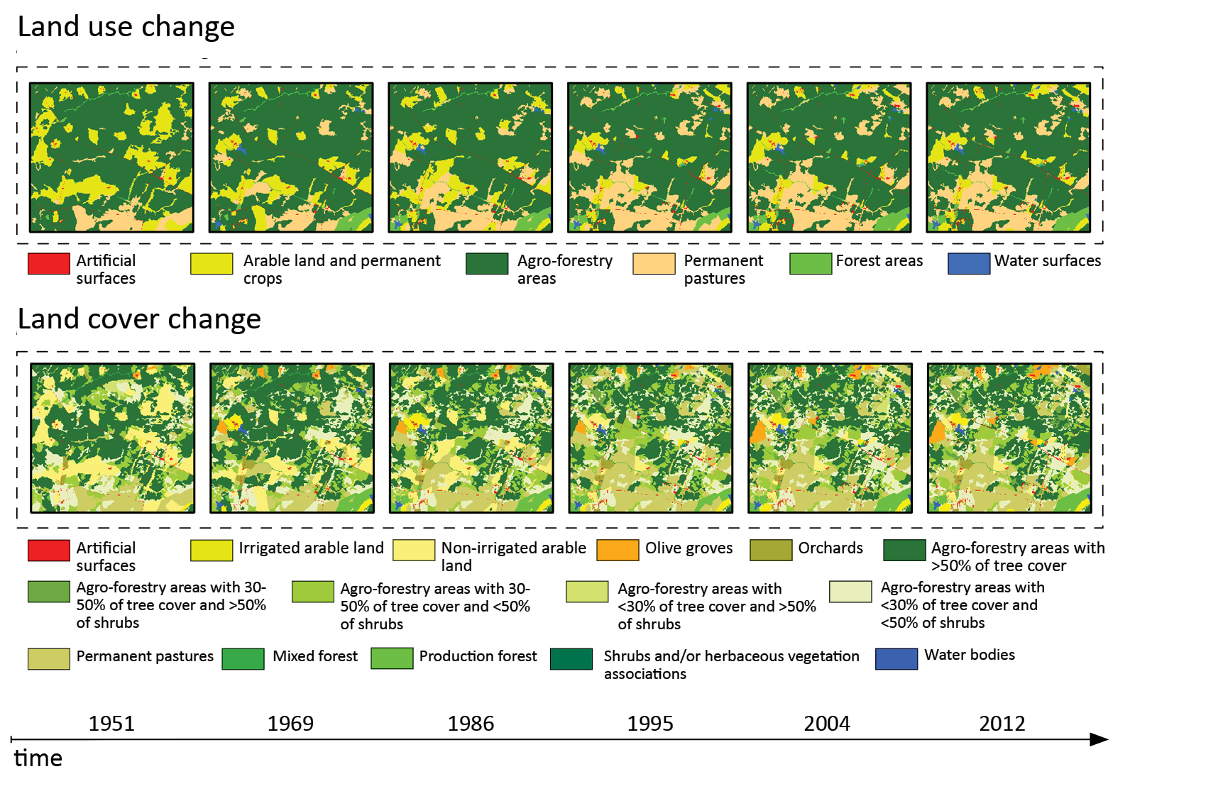
Scenario analysis
At the same time, trend analysis also presents a valuable opportunity to better design and describe future scenarios of ecosystem development. These scenarios are plausible representations of possible future states for one or more components of a system, or as alternative policy or management options intended to alter the future state of these components. Scenario analysis in ecosystem assessments, policy support and decision-making aims at visualising future impacts on biodiversity and ES of global, regional or local changes such as land use change, invasive alien species, over-exploitation, climate change and pollution. Scenario analysis also provides decision support for developing adaptive management strategies and exploring the implications of alternative social-ecological development pathways and policy options. At the same time, scenario analysis and scenario planning have been successfully applied in many local studies, in national assessment and for regional and global assessments (Chapter 5.7.3).
Generally, scenario analysis includes three major phases. The initial step is to define the major tendencies for a specific region or for a specific subject and to analyse the drivers of change that are likely to be involved in the foreseen tendencies. This phase results in a few plausible scenarios. A second phase is to translate these scenarios quantitatively or qualitatively into variables that describe the major drivers of change, such as economic development or demography. These drivers of change are then the input for models that relate these changes to environmental change, such as land use change or climate change, and on biodiversity and ES. A third phase starts with analysing the outcomes of these models and formulate policy options to avoid undesired developments in key variables of biodiversity and ES.
Models used in scenario analysis are typically able to describe dynamic relationships amongst drivers, biodiversity and ES. Often a wide range of models is needed to perform an adequate scenario analysis. Not only models that quantify changes of ES based on changes of land use are needed, but also models that drive these land use changes, such as economic and demographic models. In addition, hydrological and other biophysical models in combination with biodiversity interactions are required if more complex issues are under consideration.
New approaches for scenario analysis are proposed and applied, where stakeholders and local knowledge holders are increasingly involved. Another recent development in modelling for scenario analysis is to understand the feed-back loops from changing ES provision to a change in economic development.
Issues with data quality for dynamic assessments
Ecological modelling and particularly process-based ecological modelling, depend on a vast array of ecological, biophysical and anthropogenic datasets to generate relevant results. Although in recent years, earth observation systems have evolved to the point of delivering continuous (temporally and spatially) data for particular ecosystem components (e.g. forest change and extent, tree density, elevation, human density, economic characteristics, precipitation, etc.), many of these lack the ability to be compared or used in a modelling environment due to different resolutions and/or methods/sensors.
Additionally, there is a clear mismatch between the publication date of the variables to be used in a given assessment (e.g. LUCAS soil data from 2009) and the reference date for the assessment itself (for example using vegetation data from 2016 to assess the effect of soil erosion prevention without considering the 7 years' difference between these datasets). In several cases, if any modelling approach is to be implemented, these mismatches cannot be simply overcome and often error propagation assessments should be implemented to minimise unwanted effects.
Independently of the problems or potential caveats related to particular datasets, the temporal resolution (i.e. the amplitude and frequency of data collection) of a given dataset is an important determining factor for dataset selection in trend analysis. Therefore, future ecosystem service supply studies should include the effects of data quality on their results as it can produce important biases in the overall interpretation and decision-making support.
Further reading
- Bateman IJ, Harwood AR, Mace GM, et al. (2013) Bringing ecosystem services into economic decision-making: land use in the United Kingdom. Science (80) 341: 45-50.
- Guerra C, Metzger MJ, Maes J, Pinto-Correia T (2016) Policy impacts on regulating ecosystem services: looking at the implications of 60 years of landscape change on soil erosion prevention in a Mediterranean silvo-pastoral system. Landscape Ecology. doi: 10.1007/s10980-015-0241-1.
- Kandziora M, Burkhard B, Muller F (2013) Mapping provisioning ecosystem services at the local scale using data of varying spatial and temporal resolution. Ecosystem Services 4: 47-59. doi: 10.1016/j.ecoser.2013.04.001.
- Koch EW, Barbier EB, Silliman BR et al. (2009) Non-linearity in ecosystem services: temporal and spatial variability in coastal protection. Frontiers in Ecology and Environment 7: 29-37. doi: 10.1890/080126.
- Nelson E, Mendoza G, Regetz J et al. (2009) Modelling multiple ecosystem services, biodiversity conservation, commodity production and tradeoffs at landscape scales. Frontiers in Ecology and Environment 7: 4-11. doi: 10.1890/080023.
- IPBES (2016) Methodological assessment of scenarios and models of biodiversity and ecosystem services, Ferrier S, Ninan KN, Leadley P, Alkemade R, Acosta-Michlik LA, Akcakaya HR, Brotons L, Cheung WWL, Christensen V, Allam Harhash K, Kabubo-Mariara J, Lundquist C, Obersteiner M, Pereira HM, Peterson G, Pichs-Madruga R, Ravindranath N, Rondinini C, Wintle BA (Eds.) Secretariat of the Intergovernmental Platform for Biodiversity and Ecosystem Services, Bonn, Germany.
5.4. Why to map
Meaningful mapping
Maps for ecosystem services (ES) are made for a broad set of purposes. These include advocacy (awareness raising, justification, decision support), ecosystem assessment, priority setting, instrument design, ecosystem accounting, economic liability and scientific spatial analysis. Figure
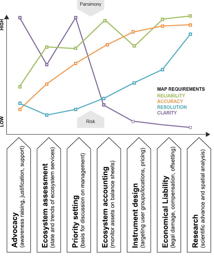
Figure
Many current mapping applications focus on quantitative valuation and accounting. Typically, these maps are neither meant to be understood by a broad range of stakeholders nor do they necessarily require a high spatial resolution, but they should be highly accurate and reliable. This chapter illustrates this for two specific examples concerning regional assessment and priority setting.
Good enough is just perfect
Mapping quality requirements are bound by resource availability and by the risk of decisions based on them. The upper boundary of requirements is set by the principle of parsimony, stating that "among two good solutions, the simplest is always best". This highlights the need for using the least resources or assumptions necessary to solve a problem. In other words, one should not spend excessive (project) time and/or (public) money to map at a greater level of detail than necessary. For example, land use based maps (see Chapter 5.6), that can be produced repeatedly at relatively low costs (in terms of time and money) are sufficiently adequate for most purposes, while more reliable data can sometimes only be obtained at excessively high cost, or involving complex assumptions. Moreover, the time spent on a specific map should be traded off against the urgency of the purpose.
The lower limit of map quality requirements is determined by the societal impact of the decisions based on the mapping. Uncertainty (or absence of information on uncertainty) translates in a societal risk for adverse outcomes if decisions are based on wrong data. Public or policy advocacy for the importance of ES does not require highly accurate or detailed maps. However, communication maps cannot be used for purposes which have more stringent requirements, such as ecosystem accounting or economic liability: the risk for unfair or undesired outcomes is too high or unknown.
This brings us to the issue of the safe operating space for each type of map. Maps with lower requirements cannot be used for purposes which have higher requirements. On Figure
Maps are means, not ends
Maps are instrumental tools that are combined with other types of data and contextual information in order to achieve a certain purpose (see Figure
The modest mapper
In this final section, we provide guidelines for critical map-makers to engage in effective ES mapping. While most of these will seem evident, they are rarely applied in practice. Following these guidelines will improve effectiveness of ecosystem service maps to impact actual decision-making and contribute to scientific advance.
- Clearly define the purpose for which mapping is needed. Plenty of maps are created without clear purpose and later applied for the wrong purpose.
- Determine the minimum reliability, accuracy, resolution and clarity required. The risk for undesired outcomes grows if maps are used for higher impact decisions.
- Assess the resources (time and money) needed to meet these requirements. Highly expensive, detailed or complex maps are not necessarily more effective.
- Delineate the safe operating space of your maps. The map-maker, being aware of the power and limitations of maps, bears responsibility to caution against wrong or risky application (see Chapter 6.4).
- Target the form and communication of maps fitted to the process they are used in. Maps are essential for many processes, but project purposes are never just maps.
ES mapping at the local scale is often used to set priorities and guide decision-making to optimise ES provision. This example describes how ecosystem service maps were combined with biophysical models and valuation data to serve a participatory land-consolidation plan for three municipalities in Wallonia, Belgium. It is co-constructed by the administrations, scientists and local stakeholders. The project's objective is to design a replicable methodology, based on hands-on experience in a first case study. Figure
After selecting a list of locally relevant ES and, based on a typology of ecosystems, biophysical assessment and social valuation are carried out. The biophysical assessment includes mapping and quantification of selected ES based on indicators obtained from a hydrological model and scenario development of potential ecosystem service supply. Social analysis comprises stakeholder analysis, societal valuation according to these stakeholders, participatory validation of the biophysically mapped ES and participatory mapping of ecosystem service demand. These supply and demand maps are then used to guide participatory comparison of land-consolidation actions. For instance, maps of biophysical indicators were compared with demand maps to highlight locations for which there is potential improvement of supply. Technical experts of land consolidation then suggest potential measures (e.g. installation of new hedgerows, creation of new water retention basins, new flower strips along a walkway etc.) to be implemented in the final land consolidation plan. This example clearly demonstrates that maps are used as a central means in combination with various other data, methods and actions, to achieve a broader objective shared by various stakeholders and lead to improved decision-making.
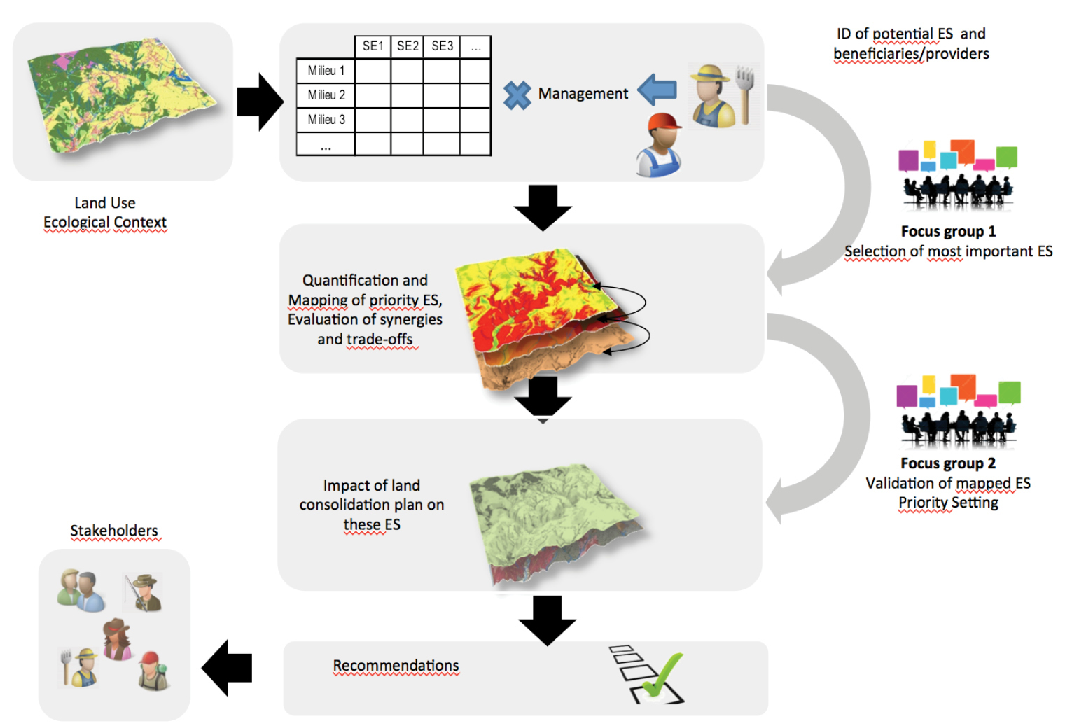
National and regional ecosystem service assessments seek to assess the state and trends of ES in their region, with the purpose of monitoring their evolution and informing policies. The state of ES comprises information on the demand, the supply, the balance between demand and supply, the use of ES, ecosystem functions underpinning them, drivers of change, impacts on human well-being and governance. Spatial data - also in regions with high data-density - are not available for all aspects of all services and for some aspects the spatial dimension is even irrelevant.
The Flanders regional assessment has assessed demand, supply, balance between these two and interactions between use of services. These statements were based on a detailed review of all data and information in 16 ecosystem service chapters to obtain one single concise table on the state of ES with known reliability. Despite the focus of the chapters on maps, the data underpinning this assessment are only partly spatially explicit and range over different data types which are synthesised in key findings (Figure
In conclusion, maps which are integrated in communication, decisions or even research will be reduced to quantitative or qualitative findings and combined with other data and information to obtain final outcomes. Mapping will be more effective when engaging in the specific context, by targeting and communicating the maps to the specific purpose and by tuning maps to the diverse information they are combined with.
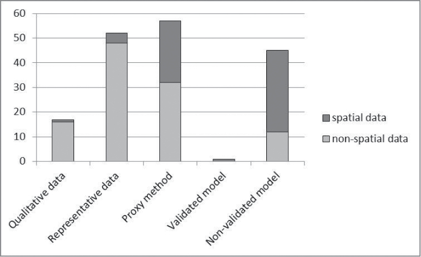
In many cases, maps are a starting point for an open discussion about what the maps need to indicate and about the assumptions made in the underlying models. Using maps top-down as 'objective data' often discards nuanced reality of a local context and is counterproductive in most real-life decision processes. To effectively apply maps, the ES map-maker needs to involve:
- Interdisciplinary engagement: learn from existing practices and cooperate with other research fields, such as environmental decision support, communication science, participatory processes, etc. to avoid classic pitfalls.
- Trans-disciplinary engagement: consider the use of co-design approaches from the very start. Nowadays, stakeholder involvement is an essential indicator for end-user satisfaction and final uptake of the developed maps and the only reality check the ES-map-maker has.
Ecosystem service mapping can be highly rewarding in terms of impact on real-world decision-making. This requires leaving the comfort zone of single disciplines and clear data layers and finding the right balance between scientific demands, user demands, functionality and available resources. for every mapping project again.
Further reading
- Baptist F, Degre A, Grizard S, Maebe L, Pipart N, Renglet J, Sohier C, Dufrene M, Dendoncker N (2016) Elaboration d'une methodologie d'evaluation des incidences sur l'environnement de l'amenagement foncier s'appuyant sur la notion des services ecosystemiques. Rapport general. Direction Generale Operationnelle de l'Agriculture, des Ressources Naturelles et de l'Environnement, 187 pp.
- Gomez-Baggethun E, Barton DN (2013) Classifying and valuing ecosystem services for urban planning. Ecological Economics 86: 235-245.
- Guerry AD, Polasky S, Lubchenco J, Chaplin-Kramer R, Daily GC, Griffin R, Ruckelshaus M, Bateman IJ, Duraiappah A, Elmqvist T, Feldman MW, Folke C, Hoekstra J, Kareiva PM, Keeler BL, Li S, McKenzie E, Ouyang Z, Reyers B, Ricketts TH, Rockstrom J, Tallis H, Vira B (2015) Natural capital and ecosystem services informing decisions: From promise to practice. Proceedings of the National Academy of Sciences 112(24): 7348-7355.
- Hauck J, Gorg C, Varjopuro R, Ratamaki O, Maes J, Wittmer H, Jax K (2013) Maps have an air of authority: Potential benefits and challenges of ecosystem service maps at different levels of decision making. Ecosystem Services 4, 25-32. doi: 10.1016/j.ecoser.2012.11.003.
- Jacobs S, Dendoncker N, Keune H (Eds.) (2013) Ecosystem Services: Global Issues, Local Practices, Elsevier, New York.
- Jacobs S, Spanhove T, De Smet L, Van Daele T, Van Reeth W, Van Gossum P, Stevens M, Schneiders A, Panis J, Demolder H, Michels H, Thoonen M, Simoens I, Peymen J (2016) The ecosystem service assessment challenge: Reflections from Flanders-REA. Ecological Indicators 61: 715-727. doi: 10.1016/j.ecolind.2015.10.023.
- McIntosh BS, Ascough JC, Twery M, Chewe J, Elmahdi A, Haase D, Harou JJ, Hepting D, Cuddy S, Jakeman AJ, Chen S, Kassahun A, Lautenbach S, Matthews K, Merritt W, Quinnm NWT, Rodriguez-Roda I, Sieber S, Stavenga M, Sulis A, Ticehurst J, Volk M, Wrobel M, van Delden H, El-Sawah S, Rizzoli A, Voinov A (2011) Environmental decision support systems (EDSS) development - Challenges and best practices. Environmental Modelling & Software 26: 1389-1402.
- Pavlovskaya M (2006) Theorising with GIS: a tool for critical geographies? Environmental Planning A 38: 2003-2020. doi: 10.1068/a37326.
5.5. Mapping specific ecosystem services
This chapter is one of the core chapters of this book. It contains guidance and examples of how to map provisioning, regulating and cultural ecosystem services (ES). These three categories constitute a commonly used classification for ES (see Chapter 2.4) and thus for ES mapping.
Different methods and models are used to map specific ES as indicators, used to quantify these three categories of ES, differ remarkably. Provisioning ES are often quantified based on indicators for their actual use/ES flow or demand (see Chapter 5.1) or their value. In contrast, assessment of regulating ES is usually based on supply indicators, such as the different ecological processes which are the basis of ecosystem regulation or avoided events (e.g. erosion or floods) and related hazards. Indicators for cultural ES have been mostly limited to recreation and (eco-)tourism for which both supply (popular ecosystems to visit) and demand (visitor numbers) are quantified.
The use of provisioning ES involves the extraction of a product from the ecosystem (e.g. harvested biomass in tonne per ha per year; see Chapter 5.5.2). Mapping provisioning ES therefore relies often on data from statistical offices which collect statistics of water consumption, crop and timber harvests, fishery yields and livestock data. Sometimes these data are geo-referenced and are thus available as geospatial data layers. If not available, statistical data can be spatially allocated over different ecosystem types, land use/land cover types or other spatial units such as watersheds or cadastral data to obtain mapped values.
Regulating ES (see Chapter 5.5.1) are often mapped by using biophysical models (e.g., ecosystem models, species distribution models, water and air quality models; see Chapter 4.4). These models simulate the fate and transport of, for example, carbon, nitrogen, water or pollutants through the ecosystems and the environment. The ecological processes which are modelled can be used to infer values for regulating and maintenance ES. Researchers mostly map potential or flow of regulating ES (see Chapter 5.1). Demand for regulating ES is usually not mapped since it is conceptually less understood (see Chapter 6.2).
As already indicated, assessments of cultural ES (see Chapter 5.3.3), to date, are mostly limited to recreation and tourism. Actual use/ES flow needs to be mapped based on surveys, national accounts and data collection (e.g. national park visitor statistics or entrance fees). These data can be combined with spatial data in order to map and assess the service and to provide detailed information on how ecosystems contribute to recreation and tourism.
The remainder of this chapter goes into more detail for each of these. Each ES categories section contains a representative selection of ES for which mapping techniques and methods are illustrated at various spatial scales.
5.5.1. Mapping regulating ecosystem services
Introduction
Ecosystems regulate our environment by controlling or modifying the stocks and flows of material and energy that make up our ambient environment. Ecosystems help provide clean air and water by removing pollutants. They regulate the global and local climate through evapo-transpiration or simply by providing shade. They maintain habitats for insects and birds which support the production of crops or which suppress pests and diseases. They store carbon, buffer flows of water or maintain the fertility of soils. All these services are not directly consumed as goods by people but regulating ES provide many direct benefits by keeping a safe and habitable environment, supporting food production systems or processing and removing waste and pollution.
Before mapping, it is important to understand first which ecosystem processes are at the basis of regulating ES and what the spatial characteristics are (scale and direction of different flows of material and energy). Furthermore, it is crucial to consider the difference between mapping capacity and mapping flow or use (Chapter 5.1). Actual use of a regulating service happens when there is a demand for it. Consider the protection of soils from erosion. Soil erosion in cropland occurs when wind or water remove fertile soils (topsoil). Vegetation, in particular grasslands and patches of forest, keep the soils fixed and thus avoid erosion. To provide the service, two conditions need to be met. First, there needs to be a demand for soil protection. Typically bare croplands on slopes are prone to erosion so farmers would benefit from enhanced capacity of the ecosystem to protect soils. Second, the right ecosystems need to be present to provide the service wherever and whenever the service is needed.
Understanding the different functions that underpin the delivery of regulating ES is thus the first step in a mapping process. In broad terms, ecosystems deliver regulating services by storing, capturing, absorbing or immobilising material such as carbon, water or pollutants, by maintaining or creating suitable conditions for species that provide regulating services (e.g. pollination, pest control, or soil quality regulation), or by buffering or mediating material and energy stocks and flows (regulation of waste and toxics, regulation of the atmosphere, water or soil erosion).
The remainder of this chapter presents detailed examples of how different regulating and maintenance ES can be mapped. We frame ES mapping using the ES cascade model (see Chapter 2.3) and classify maps depending on whether they represent ecosystem processes, functions (potential supply), use or demand. The focus is on the biophysical mapping, not on mapping economic values. For every ecosystem service, we identify each time which underpinning functions can be mapped but we also describe how to map actual use and demand.
Although this chapter does not present all methods available for mapping, it gives the reader a flavour on how to map certain regulating ES. Several other chapters provide other useful ways to map ES, for example, based on Bayesian statistics (Chapter 4.5) or matrix models (Chapter 5.6.4). The work presented here falls largely under the category of tier 3 maps (see Chapter 5.6.1). Such ecosystem service maps are based on models which are spatially resolved.
Crop pollination
Different ecosystems, particularly forest edges, flower rich grasslands or riparian areas, offer suitable habitats for wild pollinator insects such as solitary or honey bees, bumblebees or butterflies. As soon as these insects start foraging, the ecosystems that host these insect populations have the potential to increase the yield of adjacent crops which are dependent on insect-mediated pollination. Fruit, vegetables, nuts, spices and oil crops profit from pollination. Mapping supply and demand of pollination services therefore involves mapping the suitability of ecosystems or habitats for pollinator insects, mapping flight distances between the nest and the crops that need pollination (which range from a few metres to a few kilometres) and mapping the occurrence of crops in need of pollination.
Habitat suitability maps are usually based on a number of environmental layers organised within a Geographic Information System (GIS). Examples of spatial layers relevant to pollination maps are land use/land cover, topography, distance from roads, or semi-natural vegetation. The choice of layers largely depends on which data are available and on knowledge about the ecological traits of the pollinator species. Habitat suitability maps, based on literature reviews and expert opinions, involve assigning a weight to each factor and then a suitability score to each class within a factor. Suitability scores, combined with an estimated foraging distance, are then combined to form a single (habitat) suitability map. Habitat suitability maps derived from empirical or statistical techniques require species occurrence data which can be either presence/absence or presence-only records. The suitability is then derived by relating species occurrences to habitat factors by means of the chosen technique. Examples are regression methods, machine learning techniques and Bayesian statistics. Different packages and stand-alone software exist to implement these techniques; examples include packages available within the software R, or stand-alone modelling tools such as Maxent or DIVA-GIS. The results of these models are then imported to GIS software to display maps of probability of species occurrence across the landscape of interest. Suitability maps for insect pollinators, regardless of the approach adopted to obtain them, can be interpreted as supply (potential services).
Mapping the demand requires information on where crops that need pollination are grown in combination with information on crop dependency on insect pollination. Information on the pollinator-dependency can be obtained through literature and expert knowledge. Crop location, on the other hand, can be obtained through a variety of resources. Examples of these resources are regional statistics on agricultural land and production, online databases, field samples and models (for instance when looking at future potential crop distribution). The choice often depends on the extent of the area (e.g. regional vs. national vs. global data), on the crop type (e.g. perennial vs. annual) and on the agricultural practice (e.g. rotational agriculture). Mapping the use can be based on overlay of supply (i.e. the habitat suitability) and demand (i.e. the crop distribution) or based on modelling the impact on yield in the absence of pollination.
Soil protection
The root network of grass, herbs, shrubs and trees physically keeps soil together; thus, it avoids soil from being eroded by the natural physical forces water or wind and flushed downstream to cause problems such as loss of fertile soil or siltation of watercourses. The demand for soil erosion control services is usually associated with farmland dedicated to crop production on slopes. Rainfall on bare soils, for instance after harvesting, enhances erosion.
Mapping soil protection is largely based on mapping soil erosion. Five main factors contribute to soil erosion: rainfall, erodibility or soil type, absence of vegetation, slope and land management. These are usually modelled using the Revised Universal Soil Loss Equation (RUSLE) equation. By turning on or off the impact of vegetation or conservation practices, the contribution of ecosystems can be estimated to avoid soil erosion which is then taken as an indicator for soil protection or soil retention. This is quantified by means of two indicators: the capacity of ecosystems to avoid soil erosion and soil retention (actual ecosystem provision). The capacity or potential of a given land cover type to provide soil protection can be mapped with a dimensionless indicator taking values between 0 and 1. Capacity is assumed to be correlated with the amount of vegetation which, in turn, can be derived from remote sensing data such as the Normalised Difference Vegetation Index (NDVI). Soil retention can be calculated as the difference between a model which calculates soil loss without vegetation cover and a model including the current land use cover pattern. A case study on mapping soil protection is illustrated in Box
Climate regulation
Ecosystems regulate our climate at various levels. In and around cities, urban forests provide shade during hot summer days and by evaporating water through their leaves, they cool down cities, thus delivering benefits in terms of saved energy costs or lowered ozone production and concentration. On larger spatial scales, forests, wetlands, coastal systems and other ecosystems maintain comfortable atmospheric conditions and regulate climate. Yet, mapping ES which contribute to the regulation of climate, is often narrowed down to mapping carbon storage and carbon sequestration. Climate change science and policy is evidently the reason for this focus. Net primary production is at the basis of this and many other ES and therefore often mapped. Much useful information to map primary production is available through remote sensing, field observations and modelling.
Given the increase in atmospheric carbon and the consequences for climate, terrestrial carbon pools are an important factor in the carbon balance. The terrestrial organic carbon pool (soil and vegetation) is estimated to be 3500 Pg C, most of which (75%) is stored in soil. This is almost fivefold the amount of carbon in the atmosphere. The carbon stored in the soil mainly originates from dead organic material. The main governing factors for the status of the soil organic carbon (SOC) pool are land use/land cover and local climatic conditions. Changes in land use and management practices can lead to imbalances in the flux between carbon pools. Depending on environmental conditions, the SOC pool can act as either a source of atmospheric carbon or a sink, i.e. removing carbon from the atmosphere.
An assessment of soil protection in Europe in 2010: (a) Soil retention at European scale, b) Soil retention in Central Portugal, c) Capacity to avoid soil erosion in Central Portugal and d) Structural impact in Central Portugal. Soil retention (Es) was calculated as soil loss without vegetation cover (structural impact, Y) minus soil loss including the current land use/cover pattern (the mitigated impact), measured in tonns ha-1 year-1.
The structural impact is the total soil erosion impact when no ecosystem service is provided. The capacity of a given land cover type to provide soil protection (e) is expressed using values ranging from 0 to 1 for every mapped grid cell. To estimate the capacity, the vegetation per land cover type was computed using the Normalised Difference Vegetation Index (NDVI), the environmental zones and the snow cover. The highest soil retention values corresponded to areas covered by forest, transitional woodland and shrubs (semi-natural vegetation areas) and pastures.
Soil retention is also a function of structural impact (high potential erosion). Expressed differently, soil retention only occurs where soils run the risk of being eroded. In these places, vegetation cover protects the soil against water flows (surface runoff), reduces the structural impact and, therefore, effectively delivers a service.
A close up is presented for the central part of Portugal (Alentejo and Centro Regions). In the Tagus river valley, soil retention is low (light orange areas) due to a low structural impact and the dominant land use type, mainly agriculture. High soil retention (high provision of the service, in dark blue) results from the combination of high structural impact and high capacity to avoid soil erosion, for instance in forested areas. In contrast, if the inherent structural impact is low, the provision of the service (soil protection) is low as well, thus lowering the role of vegetation in soil protection.
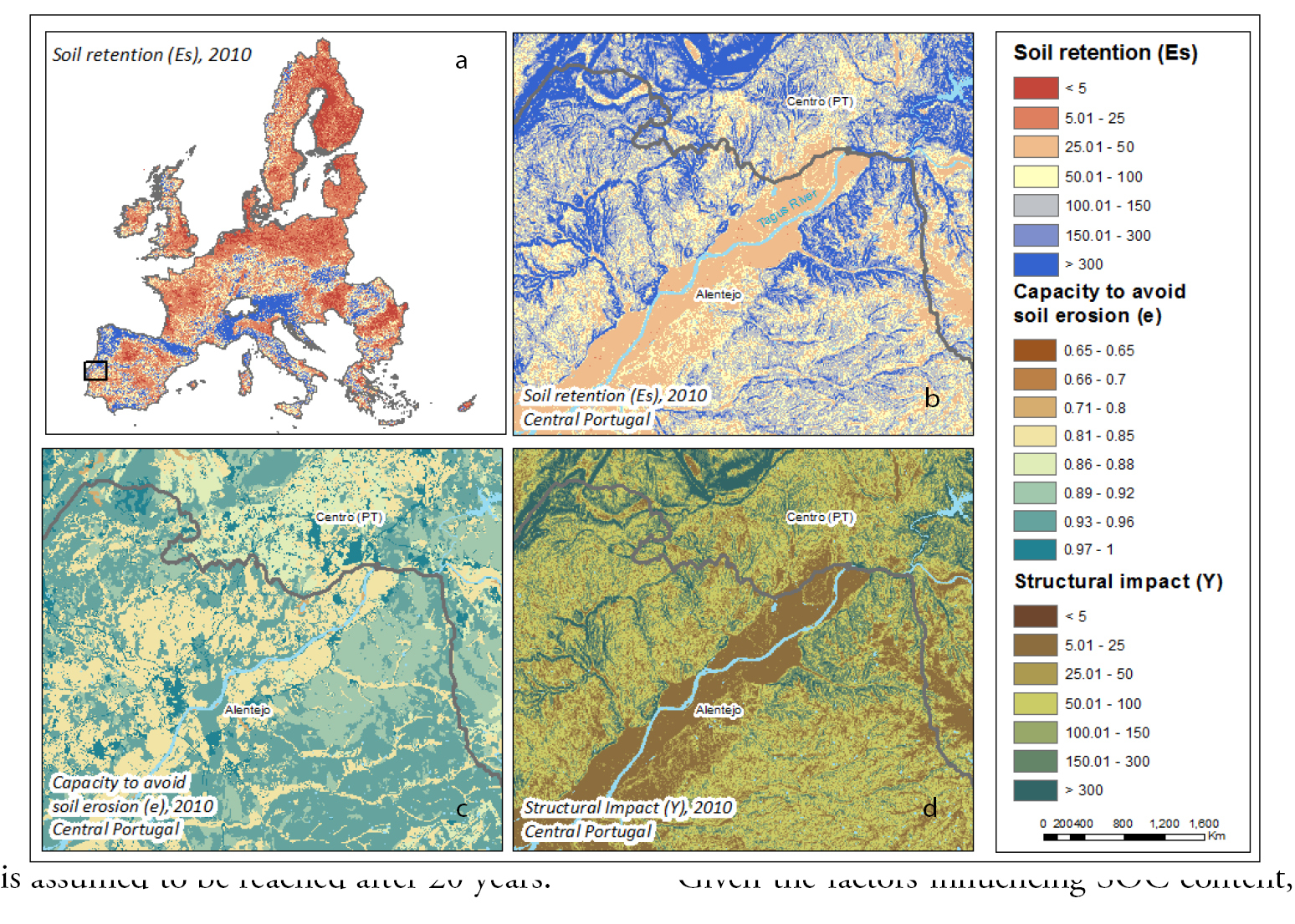
Mapping changes to the SOC pool can be based on the methodology of the International Panel on Climate Change (IPCC). The method uses type of climate, soil, category of land use, management and input practices as factors influencing SOC stocks. For each factor, the relative effect of changes to the SOC pool is provided for different climate/soil regions. When all factors remain unchanged, an equilibrium in the SOC pool is assumed to be reached after 20 years.
Given the factors influencing SOC content, the spatial distribution of SOC stocks is very variable (Figure
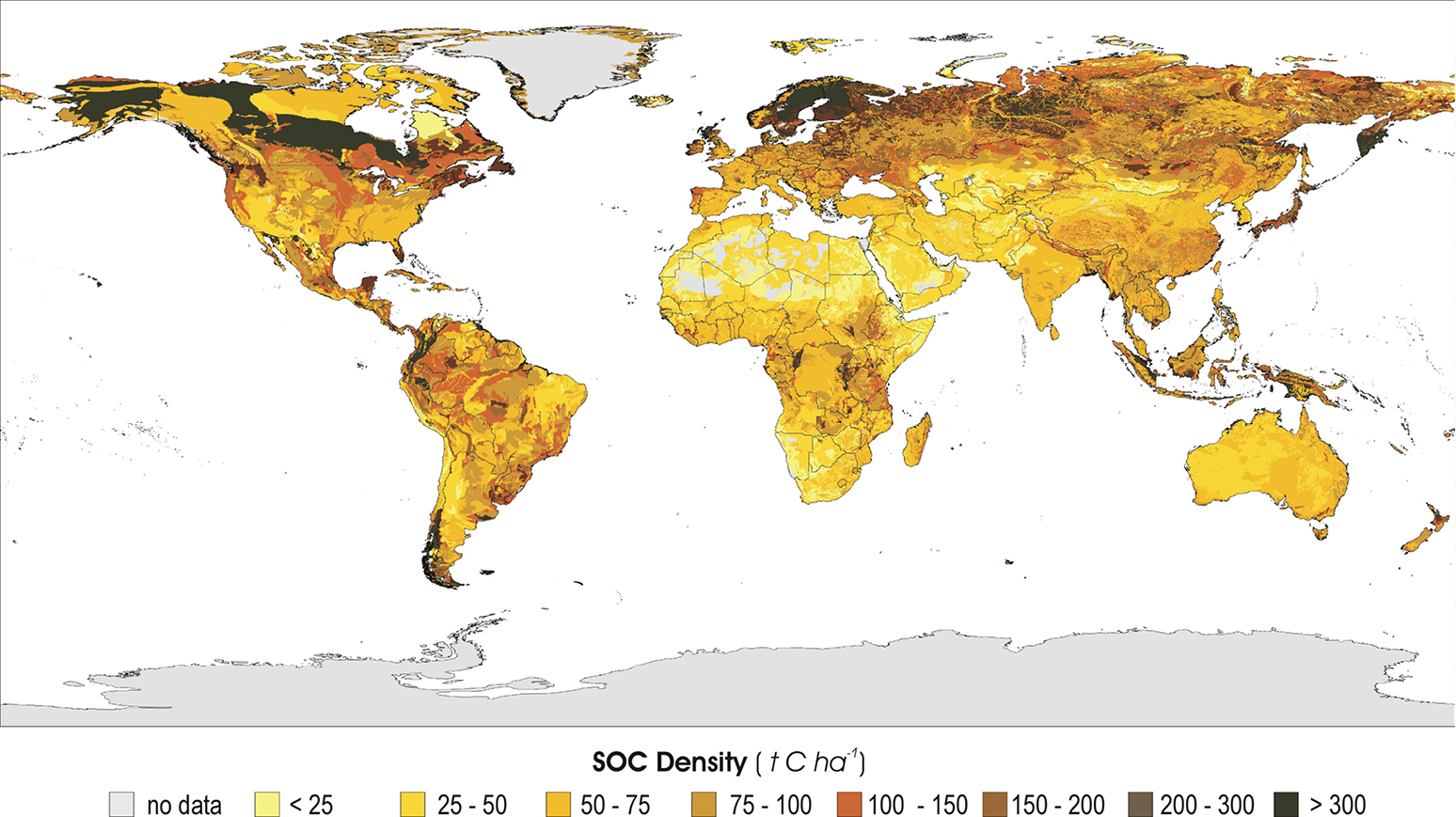
Water regulation
Forests, grasslands and wetlands are ecosystems with a high capacity for regulating the flow of water. This is particularly important for ensuring the supply of a sufficient quantity of water to support the immediate environment whilst avoiding extreme fluctuations in water flows. Where water is not properly regulated by the ecosystem (e.g., in cities, where the natural water cycle is often interrupted by impermeable surfaces), there is a much higher risk of such fluctuations, potentially leading to flooding or water shortages. The provision of water regulation can be mapped by breaking down the process into its various components. Ideally, the landscape should naturally retain and store an adequate amount of water for its needs, whilst limiting the amount of surface runoff - an excess of which may cause flooding further downstream. Water flow through a landscape may be influenced by the following natural processes, all of which contribute to the storage of water and therefore the reduction of surface runoff: interception by vegetation, storage in surface water bodies, infiltration and retention in soil and percolation to groundwater stores.
In addition to these processes, the amount of water which can be retained will also be affected by the slope of the landscape and by the degree of permeability of the soil. Steeper slopes will promote faster surface runoff, whilst flatter areas allow greater time for infiltration of water. Impermeable surfaces (e.g. artificial infrastructure such as roads and buildings) represent a barrier to the infiltration and retention of water, thus promoting surface runoff.
Figure
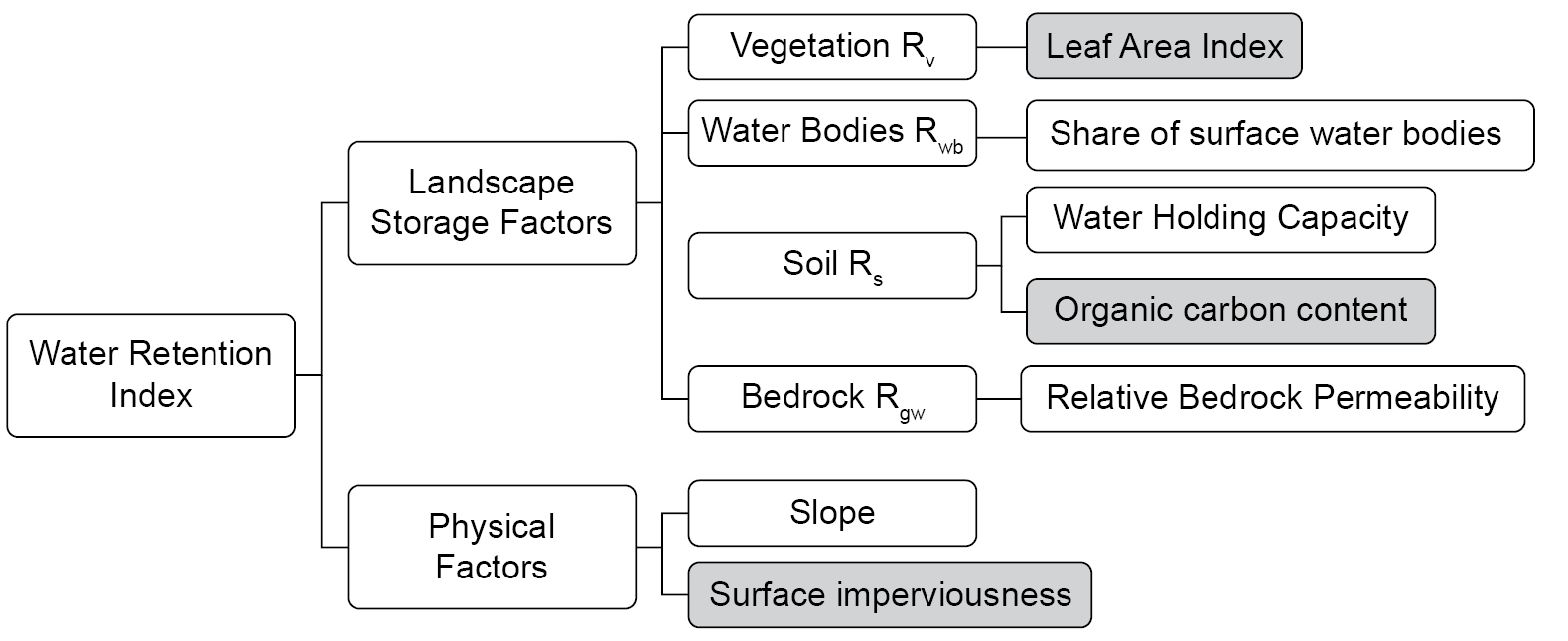
Schematic overview of the structure of the indicator for mapping water retention. Parameters in grey are dynamic and thus change over time.
The retention of water in vegetation, surface water bodies, soil and bedrock (groundwater stores) are considered landscape storage factors. Additionally, the influence of slope and surface imperviousness are considered as physical factors altering the actual water retention capacity of the landscape. The contribution of each process to the final indicator is approximated using one or more parameters or characteristics of the landscape. The parameters shaded in grey are those which are changeable over time. The various factors are combined to give the final composite indicator representing relative landscape water retention or, rather, the capacity of the ecosystem to provide water regulation as a service.
Pest control
Agricultural ecosystems are often harmed by pests such as insects (i.e. caterpillars) and small mammals (i.e. moles), significantly reducing the harvested share of crop production. However, nature offers natural fighters against these pests, thus saving farmers billions of dollars annually by protecting crops and reducing the need for chemical control. There are different groups of natural enemies known to play a key role in pest control, such as birds, mammals, spiders, lady bugs and other types of organisms. So, mapping pest control clearly relies on spatial information on the distribution of predator species (species distribution models, see also section on pollination).
We show below an example of mapping potential pest control by birds in agricultural systems (Figure
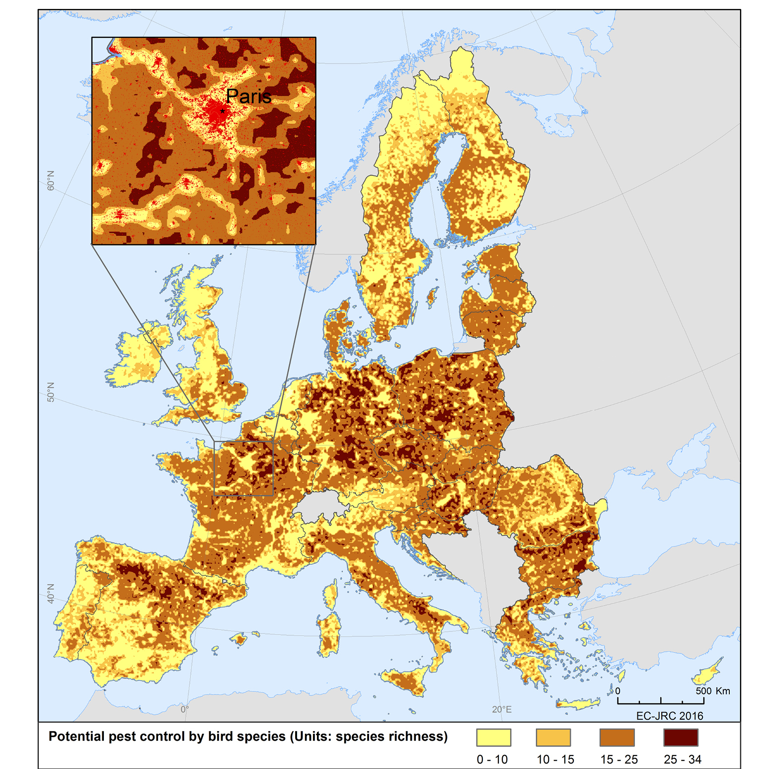
Spatial distribution of predatory bird species richness in the European Union. The close-up around Paris shows that species richness is lower near urban areas (mapped in red).
Species distribution models map the probability of species occurrence based on field observations. A probability threshold can be defined for instance at 50% to assume the presence of a certain species. By overlaying all the species occurrence maps of the 49 modelled species, a map of potential pest control by predatory birds is obtained. Higher species richness corresponds to a more diverse community of natural predators and is assumed to exert a greater control on pest populations. Figure
Air quality regulation
Air pollution is one of the main environmental risks for human health and is the main cause of premature deaths. In this context, abatement of pollution has become of major concern especially in areas with high pollutant concentrations, typically urban areas. Maintaining and developing green urban areas can be part of an integrative strategy to help increase air quality in European cities. Trees reduce temperatures in cities by evaporating water and they remove air pollutants and particulate matter via their leaves through dry deposition. Urban trees, green areas and forests surrounding cities have the capacity to remove significant amounts of pollutants thereby increasing environmental quality and human health.
Mapping air quality regulation is based on three types of information: the dry deposition velocity (supply), the removal of air pollutants (flow) and human exposure (demand).
The pollutant dry deposition velocity by vegetation is considered often as a proxy to assess the ecosystems capacity to remove pollutants from the atmosphere. This quantity measures the rate at which pollutants are collected from the atmosphere by tree leaves. The contribution of vegetation is often mapped and modelled using spatially explicit data of the leaf area index (LAI). The LAI is defined as the one-sided green leaf area per unit ground surface area. The larger this area, the more pollutants are captured by trees.
Furthermore, the pollutant removal flux by vegetation, which is estimated as the product of pollutant dry deposition velocity by vegetation and pollutant concentration, is usually considered as a good measure for the ecosystem service flow.
Finally, demand for the service can be mapped using population exposure to pollutant concentrations beyond the limit established within the legislation currently in force.
Maps of the atmospheric concentration of pollutants are essential inputs to map air quality regulation as an ecosystem service. Mostly, they rely on a network of monitoring stations where different pollutants are measured. The measurements collected by different monitoring stations can then be interpolated to obtain maps of concentrations. Several GIS techniques exist to perform interpolation by, for example, kriging and spatial regressions.
Figure
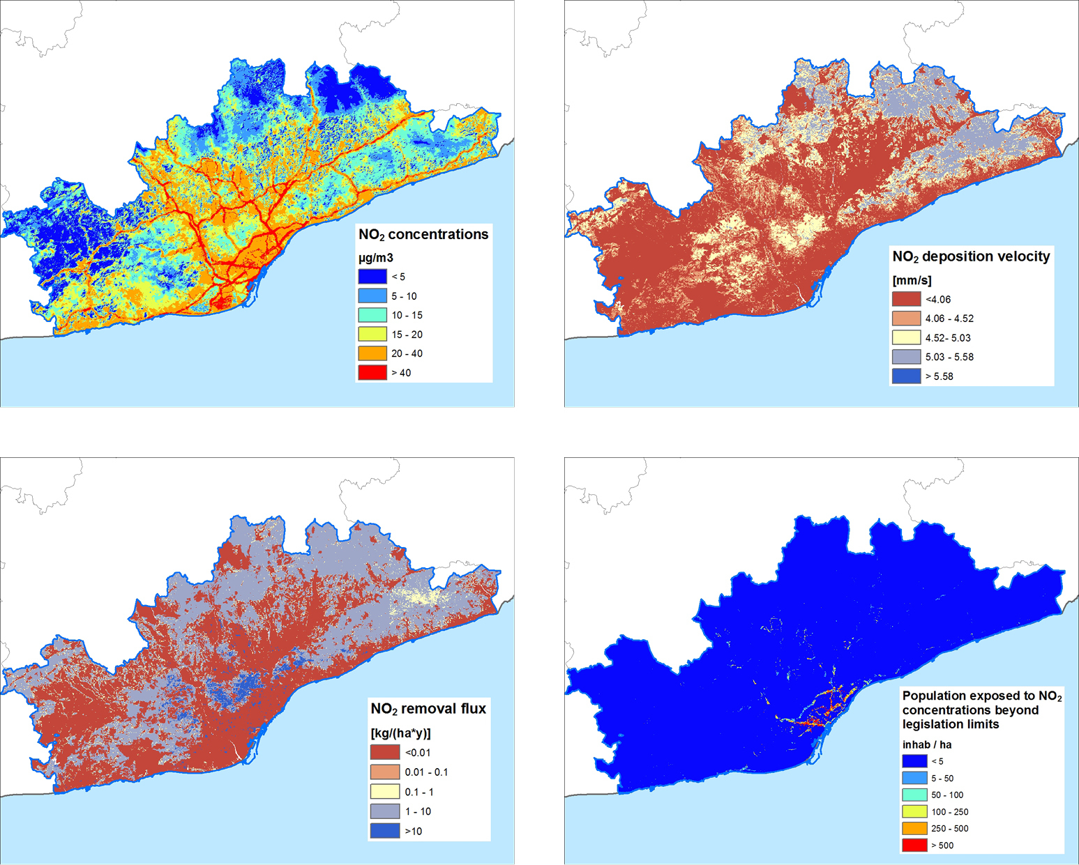
Conclusions
Much progress has been achieved in mapping regulating ES. Data, maps and models are often available from other scientific disciplines such as research on air quality, hydrology, climate change or biodiversity and they need relatively minor adaptations for applications in an ES context.
Mapping regulating ES is often based on mapping the capacity of ecosystems to provide these services rather than mapping the actual use of the service. One possible reason is that it is not always clear what the use is of a regulating service in comparison with provisioning services.
Mapping the capacity of ecosystems to provide regulating services can be based on the combination of different data layers to arrive at a composite index between 0 and 1 where 0 stands for no capacity to deliver a service and 1 stands for maximum capacity. Where species provide a regulating service, capacity is often approximated based on species occurrence which can be mapped. In the case of air quality regulation, mapping capacity is based on mapping the dominant physical process (deposition).
The case of soil protection demonstrates how actual flow or use of regulating services can be done. Avoided erosion is modelled as the difference between erosion in the absence of vegetation and erosion with protective cover. This technique can be applied to other regulating services such as pollution and excess nutrient control.
Demand for regulating services can be mapped if spatial data are available which identify use, users or beneficiaries. Examples are crops which need pollination, farmland exposed to erosion or people exposed to low levels of air quality.
Further reading and resources
- Civantos E, Thuiller W, Maiorano L, Guisan A, Arajo MB (2012) Potential impacts of climate change on ecosystem services in Europe: The case of pest control by vertebrates. BioScience 62: 658-666.
- FAO and ITPS (2015) Status of the World's Soil Resources (SWSR) - Main Report. Food and Agriculture Organisation of the United Nations and Intergovernmental Technical Panel on Soils, Rome, Italy, 650 pp.
- Guerra CA, Maes J, Geijzendorffer I, Metzger MJ (2016) An assessment of soil erosion prevention by vegetation in Mediterranean Europe: Current trends of ecosystem service provision. Ecological Indicators 60: 213-222.
- Nowak DJ, Crane DE, Stevens JC (2006) Air pollution removal by urban trees and shrubs in the United States. Urban Forestry and Urban Greening 4: 115-123.
- Polce C, Termansen M, Aguirre-Gutierrez J, Boatman ND, Budge GE, Crowe A, Garratt MP, Pietravalle S, Potts SG, Ramirez JA, Somerwill KE, Biesmeijer JC (2013) Species Distribution Models for Crop Pollination: A Modelling Framework Applied to Great Britain. PLoS ONE 8: e76308.
- Scharlemann JPW, Tanner EVJ, Hiederer R, Kapos V (2014) Global soil carbon: Understanding and managing the largest terrestrial carbon pool. Carbon Management 5(1): 81-91.
- Zulian G, Maes J, Paracchini M (2013) Linking Land Cover Data and Crop Yields for Mapping and Assessment of Pollination Services in Europe. Land 2: 472.
5.5.2. Mapping provisioning services
Introduction
Material and energy outputs from ecosystems are usually classified as provisioning services. These are tangible goods or services that are directly used, traded or exchanged by all human beings. They can be grouped into nutrition (e.g. cultivated crops, seafood from aquaculture, wild food), materials (e.g. fibres and genetic materials) and energy services (e.g. fuel wood). Some of them, such as cultivated crops and animal outputs, are amongst the most mapped ecosystem services (ES), whereas others, such as genetic materials and energy provided by animals, have been studied or mapped less frequently to date (Figure
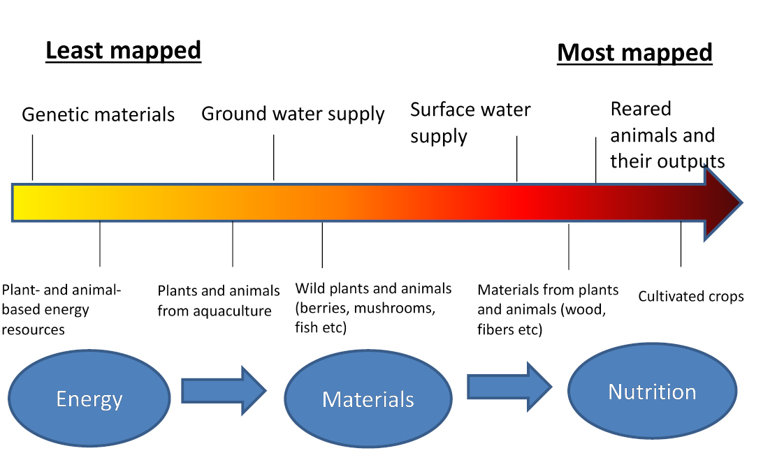
Provisioning services are often produced and consumed or used in different places. They are generally transported from the place of production (i.e. supply) to the place of consumption (i.e. demand). It is more common and easier to map the supply, as it is spatially explicit and directly depends on the ecosystem's structure and functioning, whereas the demand is a function of socio-economic drivers.
The economically important crop and animal products, as well as timber and fish products, can be closely associated with agriculture, forestry and fishery/aquaculture and consequently, their related land cover/use types. As they represent traditional economic activities and research focuses that have existed for a very long time, a large body of subject-specific knowledge and data sets are available to quantify ES supply based on these economic sectors. This fact also gives the opportunity to analyse changes and trends of these ES in many regions. These production systems are usually monocultures and require a large amount of human input (Chapter 5.1). On the contrary, wild plants, water and genetic resources are less clearly associated with one specific land cover/use class and are generated in more diverse and semi-natural or natural ecosystems and landscapes.
The production of ES is not only location-specific, but it is also dynamic over time (Chapter 5.3). Examples include crops mainly being grown and harvested in spring-summer period in the temperate zones. In the tropical zone, the growing season lasts all year around. Another example is the dynamic supply of drinking water from mountain regions, which follows the seasonal changes in hydrological and climatological conditions.
Mapping methods for provisioning services
Based on the CICES classification (Chapter 2.4), provisioning services can be grouped into the classes reported below. Different methods and data sets are available for mapping these classes. A short overview of selected mapping methods and data sets is provided in the following sections.
Cultivated crops & reared animals and their outputs (e.g. cereals, vegetables, meat, milk)
These provisioning services are mainly commercially valued and traded as the direct output of agriculture from arable land and pastures. They are amongst the best monitored ES and their level of production is documented in agricultural statistics or accounting in many areas. Therefore, they can be easily mapped using land cover/land use maps in combination with indicators of crop or animal production (e.g. t/ha/year crop yield, number of animals/ha, l/ha/year milk production) from national or other statistics. This corresponds to a tier 2 mapping approach (see Chapter 5.6.1). This method has minimal data requirements and is therefore easy and quick when the corresponding data are at hand. With such data sets, maps for these provisioning services can be generated for local up to global scales. Use of a single indicator, however, neglects the effects of the management regime and the environmental characteristics of the agricultural ecosystem (e.g. soil texture, climatic and hydrological conditions), all of which influence the level and quality of ES generated. It is also possible to include anthropogenic system inputs and environmental effects as indicators instead of only crop yield or animal numbers. Due to the commercial character, there is a large additional input (e.g. fertilisers, pesticides) in most agro-ecosystems. Furthermore, it is important to notice that in the case of reared animals, land cover/land use does not automatically correspond to the area of supply. Livestock is often kept in buildings, resulting in point accumulation within the respective map.
There are also crop or animal production models (e.g. Common Agricultural Policy Regionalised Impact (CAPRI) model or Agricultural Production Planning and Allocation (APPA) model) accounting for the ecosystem's capacity, environmental effects and human inputs to obtain more accurate results. Nevertheless, these models are time and data intensive. They are suitable if the aim is to better understand a certain production system or create a crop and animal production map for a certain location under a specific socio-economic scenario or environmental constraint.
For general purposes and the mapping of multiple provisioning services, look-up tables are in common use (Chapter 5.6.4). For some outputs from reared animals (meat, milk), only aggregated or average data exist (slaughtering for a defined reference date).
On the local scale (e.g. farm), detailed analyses can be included in maps, such as variations over a season. Considering the growing season of cultivated crops, the supply does not always match the continuous demand. Over the entire growing season, up until the moment of harvest, crops can be considered as only potential provisioning services. The real use (flow) is connected to harvest, processing and consumption.
Wild plants and wild animals and their outputs (e.g. wild berries, mushrooms, water cress, game, fish, honey from wild bees)
This class includes both commercial and subsistence berry and mushroom collection, fishing and hunting for food. These less marketed ES can provide subsistence especially in less developed countries, while they are considered by some stakeholders and researchers as hobby or recreational activities in other regions. Only few examples exist for the mapping of these provisioning services because of their individual character. Statistical data are available for hunting and recreational fishing in some regions or countries. Data and information are often available for commercial fishing as regulations (e.g. exclusive economic zone and catch quota) have to be respected in many regions. However, mapping the exact area of where fish and seafood are extracted includes uncertainties due to the mobility of most species. Mapping fishing grounds requires GPS data or interview data. Usually, statistical data are grouped into specific areas (e.g. Baltic Sea or North Sea) or on an administrational level (e.g. states and countries) making the mapping less spatially explicit. For some individual or subsistence activities, such as berry/mushroom picking, recreational fishing or hunting, licences are needed. This can be used as a proxy to quantify the amount of potential users. Most important though, is the exact area of supply and the respective amount of provisioning service. This requires laborious and possibly expensive, field studies and interviews. Data from random sampling is often used for extrapolation. Methodological studies need to reveal which natural and socio-economic settings, extrapolation or value-transfer are accurate enough for reliable results.
Mapping of berry and mushroom collection and game hunting is possible by combining land cover/land use and species habitat maps with other biophysical layers (e.g. management intensity, climatic factors) and with accessibility or travel time from settlement areas. Another approach is participatory mapping (Chapter 5.6.2) of indicators such as kg/ha berries collected or the location of honey collection, relying on the knowledge and wild food collection habits of local inhabitants and stakeholders. Wild food collection is also closely related to cultural services (such as cultural diversity and traditions) and is affected by the human-environmental relationship and societal conditions (e.g. laws, regulations, property rights). This information can be included in the mapping processes through, for example, overlaying protected areas or area with restricted access. Figure
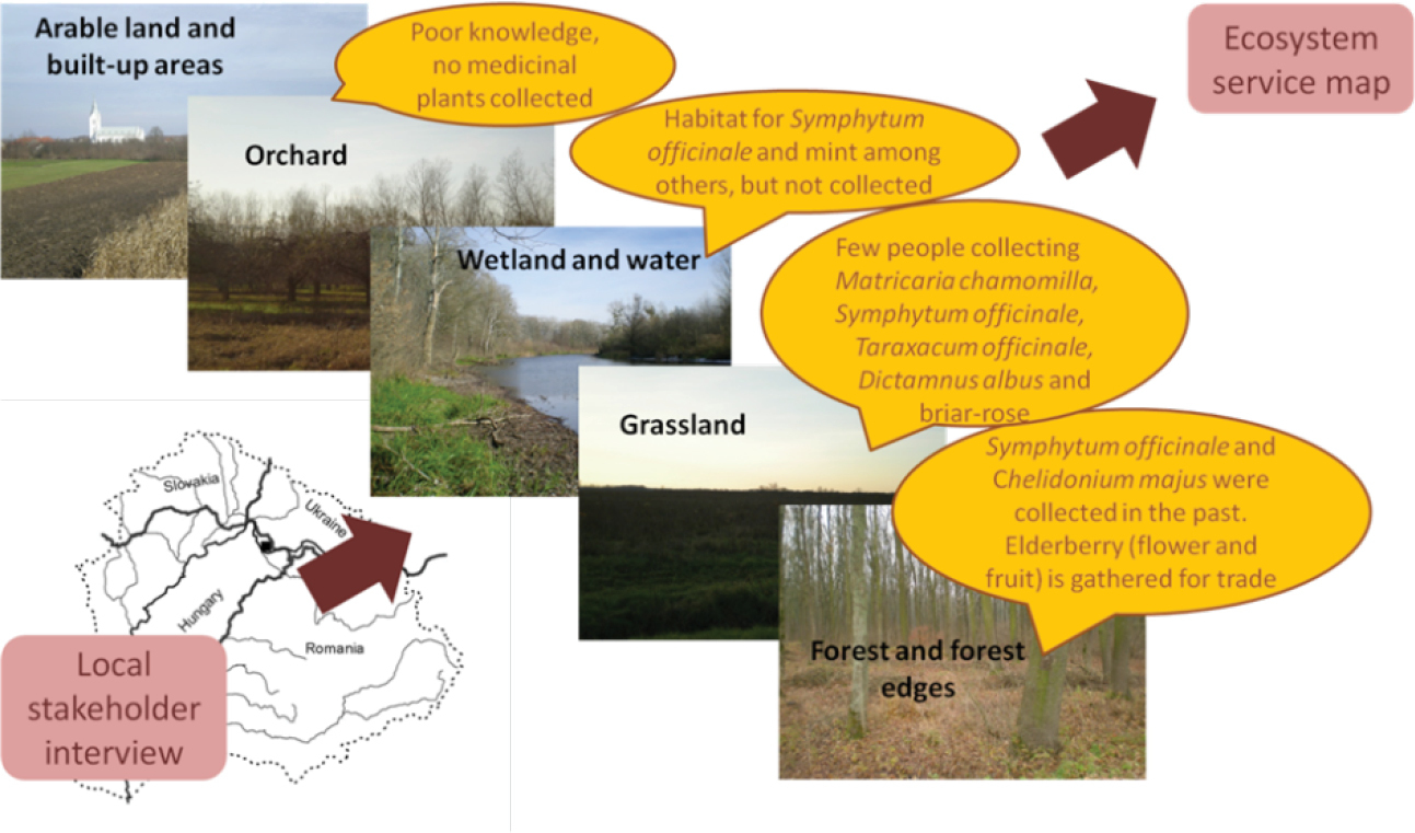
Participatory mapping of medicinal plants in the Bereg region, Hungary: Local stakeholders were questioned if, where and which medicinal plants grow and if they are collected. The growth and collection of medicinal plants were related to different land cover types. Although, the study's objective was an assessment of ES, the results could be translated into a map showing the location of this provisioning service in a further step (Source:
Few studies are available on regional or national scales. Mapping of these services (except commercial fishing) is most suitable for the local or regional scale, making it possible to include high resolution data and information needed for sustainable management.
Fibres and other materials from plants and animals (e.g. timber, cotton, grass as fodder)
This class includes both consumptive and ornamental uses and both commercial (e.g. industrial timber production) and subsistence (e.g. local wood collection) uses. Timber, grass and fodder production have been widely mapped, whereas other materials, such as cotton and silk are rarely mapped. Mapping methods range from the use of a single indicator (e.g. m3/ha wood harvested, kg/ha grass collected) to complicated forest or vegetation production models e.g., the European Forest Information SCENario Model EFISCEN (see Figure
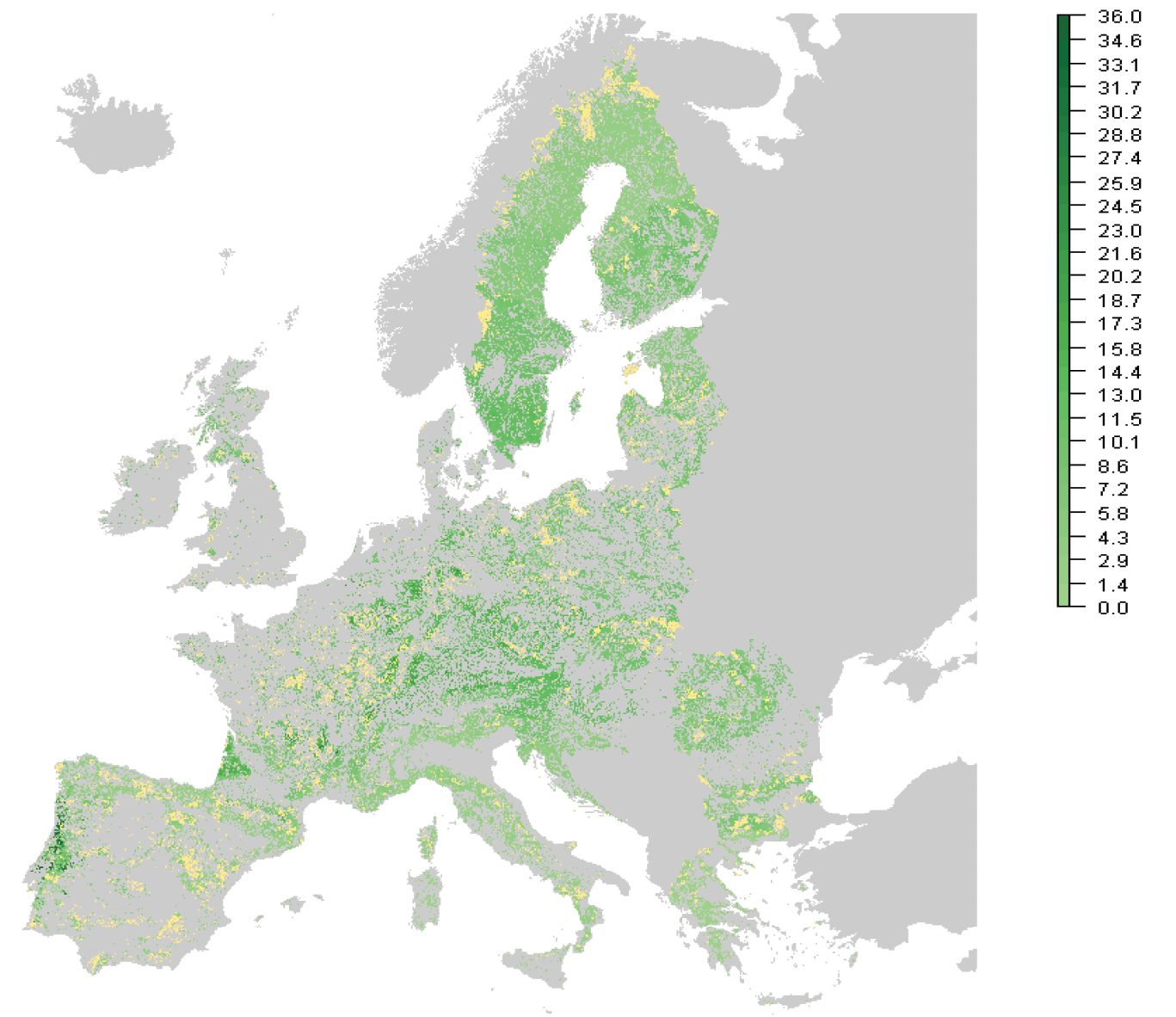
Mapping timber harvest (m?/ha/yr) in 2050 under the VOLANTE A2 business-as-usual scenario modelled with the EFISCEN (European Forest Information SCENario) model on the European scale. Yellow indicates no harvest and grey indicates non-forest areas on the map (Source: Schelhaas & Hengeveld pers. comm).
local fuel wood supply is shown in South Africa in Figure
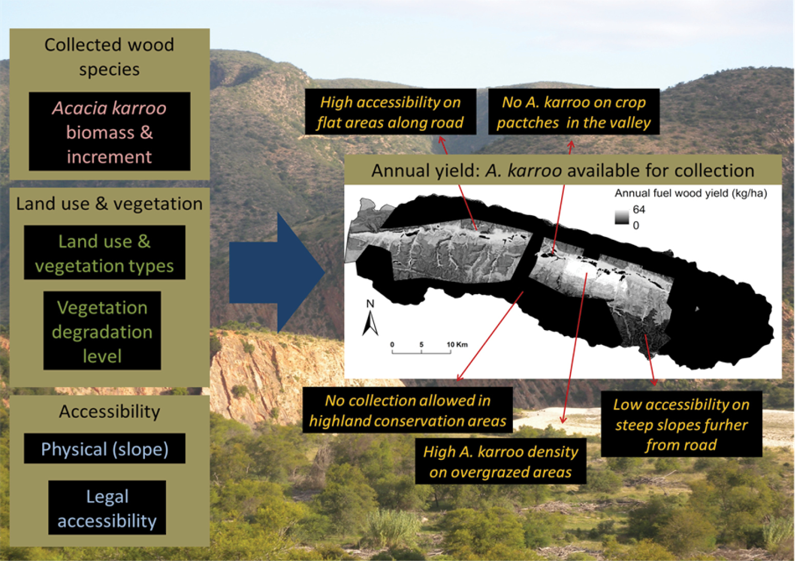
Mapping fuel wood supply in the Baviaanskloof Catchment in South Africa using local data consultations. Combining multiple indicators (left) results in a fuel wood yield map (right). Several data sets were combined to show the spatially diverse supply of fuel wood (including topography, accessibility and also conservation areas), (Source:
Similarly with cultivated crops and reared animals, there is a mismatch between the supply and demand for (some of) these services, as timber and wood products are marketed across the globe. Some fibres (e.g. cotton) belong to the most important provisioning services and are heavily traded globally. Very few studies in the context of the ecosystem service concept exist, although some (global) statistics on production are available. Recycling and multiple uses or purposes of materials result in possible uncertainty of these assessments.
The provisioning services of cultivated crops, reared animals and their outputs and materials from plants and animals are often produced on the same farm. In this case, double-counting is possible. Nowadays, fodder is however imported to many intensive farming regions, making the assessment of provisioning services more difficult or uncertain. Local mismatches of supply and demand result from this, which make the mapping of these services incomplete.
Genetic materials from wild plants and animals (e.g. medicines and wild species used in breeding programmes)
Genetic material from wild plants can be used for biochemical industrial and pharmaceutical processes (e.g. medicines, fermentation), as well as bio-prospecting activities (e.g. wild species used in breeding programmes). Genetic materials have been mapped infrequently. On a similar basis, wild food and medicinal plants have also a close link with cultural traditions and societal conditions. The occurrence or supply of medicinal plants could be mapped similarly to wild food by combining species richness and land cover/land use data or applying participatory mapping studies. Biodiversity models could provide useful information about the occurrence of different wild species. Suitable habitats for and spatial dynamics of mobile species, such as insects or mammals, can be explored with agent-based models (Chapter 4.4).
These provisioning services have been rarely mapped, although there is ongoing research (considering different species and ecosystems ranging from the tropical rainforest to marine environments). Usually, this covers only limited areas.
Animals and plants from aquaculture
Mapping provisioning services from aquatic ecosystems is usually more difficult. Information on water bodies is often not as detailed from land cover/land use maps as for terrestrial ecosystems (see Chapter 7.4). More detailed information about protected areas, different habitats, or spawning areas is needed to map animals and plants from aquatic ecosystems. An application example for mapping fishery areas in the Baltic Sea is shown in Figure

Mapping fishery areas in coastal ecosystems of the German Baltic Sea. The example shows that a land cover based approach results in an over-estimation of supply area. Here additional information is included to depict spatially explicit areas of restriction due to protection within a National Park. Boat traffic is partially prohibited. Temporal fishing restrictions exist in the spawning areas. Recreational fishing (at land) is only allowed in the designated spots and areas where boat traffic is allowed.
Wild caught fish in marine and freshwater ecosystems is an important food resource globally. Due to declining stocks and regulations (e.g. EU fisheries regulations) aquaculture is employed more and more to meet the demand for seafood and algae.
These data are available on different spatial scales and, in most cases, over a very long time period as they are important for the economy. Here also single indicators (e.g. fishing statistics in t/year) are available. Infrastructure from aquaculture, such as cages, basins, ropes, is visible in the field and can be used to identify the extent of the provisioning area.
Water for drinking and non-drinking purposes
Water extraction is usually undertaken in single spots where the conditions are suitable (i.e. infrastructure and water quantity, quality and intensity). Groundwater is recharged over a larger area and depends on ecosystem conditions, such as substrate and vegetation cover. Surface water is used in many regions where ground water extraction conditions are not suitable.
Maps can show groundwater yield and the amount of water (m3) that can be extracted without declining the yield. Hydrological models can be applied to simulate the effects of changes in consumption and hydrological and climatic conditions (Chapter 4.4).
Some statistical data are available for average water consumption (drinking water, non-drinking water) and the water incorporated or locked in products (e.g. food, clothes). Large regional mismatches occur on the global scale due to trading of products. The price for water could be used as an indicator for mapping as well.
Temporal changes in water demand is an important aspect in management, especially in areas with high usage (e.g. from tourism). In some cases, water needs to be pumped from other areas to fulfil the demand. These regional and temporal mismatches make mapping of water as an ES challenging.
Plant and animal-based energy resources (e.g. fuel wood, crops and labour provided by animals)
It is more common and easier to map plant-based energy resources than animal-based ones. The mapping of energy crops, such as oilseed rape, is similar to food crops. Sometimes they are also competing in cultivated areas.
The supply of fuel wood can be mapped with a single indicator (e.g. forest areas, occurrence of certain tree species), forest production models (e.g. EFISCEN, G4M) for commercial use and participatory approaches for subsistence use. Large regional differences exist. In some regions, fuel wood is the only energy source for cooking and heating whereas, in other regions, it is only a supplementary source or even unnecessary (e.g. urban areas with good energy infrastructure).
Labour provided by animals as an ES has not been mapped yet. It could be mapped, for example, using statistics involving the quantity of animals. In some areas, labour provided by animals is important in agriculture, but also for transportation. However, due to mechanisation in many sectors, this provisioning service is of less and less importance.
Challenges and solutions for mapping provisioning services
There are several maps and data sets available that facilitate the mapping of provisioning services. As usual, all methods have advantages and disadvantages regarding uncertainty and the objective/purpose of the maps (see Chapter 6).
When using statistical data, the maps are not always spatially explicit. These data sets are often generated at administrative levels (e.g. municipality, regions), which do not necessarily match the case study area. Although farm land might be stretched over several administrative units, the respective data (e.g. number of animals, yields) are only assigned to the location of the farm. Additionally, wild animals which hunt and fish are mobile and forage in areas which do not always match with reporting units.
Furthermore, when using statistical data, it is often not possible to distinguish between the different uses of the product (e.g. rapeseed for human nutrition, biodiesel or fodder).
Many provisioning services are supplied in larger areas that can be represented by polygons. However, there are sometimes important (hot) spots which affect only parts of an area. Besides static services providers (e.g. forests), there are some mobile ones, such as fish and seafood (see Chapter 5.2). Though the ecosystem might be restricted to aquatic ones, there are several factors that might determine the size of catches (e.g. in recreational fishing) or the exact location of the actual service (e.g. exact location of caught fish).
Temporal aspects are generally difficult to integrate on a map but several maps can be used to show the change of the supply or demand of the provisioning service over time (i.e. seasonal maps; see Chapter 5.3)). Maps on wild food (mushrooms and berries) can change significantly between years due to climatic variations or silvicultural management.
The quality of the modelling results depends on the input data and the research questions. All participatory mapping approaches are impacted by the number of stakeholders and their background and how they are instructed.
Following the grouping and classification of provisioning services from CICES, it becomes clear that the main challenge is the large and detailed amount of possible provisioning services supplied in an area or demanded by consumers. Globalisation makes it more challenging to track down detailed information on a spatially explicit scale. For many of the examples of provisioning services at the CICES class level, no data or information exist or the ES are part of a larger supply chain. Therefore, the map-maker must carefully decide to which detail provisioning services should be analysed or if a distinction into broader classes is necessary (e.g. wooden biomass from forests instead of subdividing into type and use, such as cellulose, timber, fuel food).
The question of the purpose of the map and the necessary details are also relevant. For a coarse (first) mapping of provisioning services, data sets and methods are available from local-global scale, especially when land cover/land use and statistical data can be used. The specific (policy) question guides the work and detail needed to create a proper map of provisioning services (Chapter 5.4). For the least mapped services, direct mapping based on sampling can overcome the lack of suitable data.
Another challenge is that many provisioning services outside of markets, which are mainly for private use/subsistence, have no detailed or comprehensive data sets for proper mapping. Many people are not aware of these "benefits", such as ornamental use, and do not keep detailed records or data sets. This also applies for mushroom or berry picking, or recreational fishing for personal consumption. What is most important in this circumstance, is raising awareness to show the interlinkages of ES and the need for near-nature ecosystems for the supply. The purpose and importance of these provisioning services need to be taken into account to decide whether or not a provisioning service should be classified as cultural ES or not.
The main challenge of incorporating the temporal dynamics of provisioning services in maps remains. Many studies are limited to a conceptual description of mapping provisioning services. A larger body of applications for all provisioning services would result in progress in closing the knowledge gaps, which lead to incomplete assessments of ES. A final question remains: should we map the area and spatial extent of provisioning services, which is comparatively easy with land use/land cover maps, or should we also include information on the amount, quality and benefits?
Conclusion
Maps of provisioning services are essential, as provisioning services play a key role in economic activities from local to global scale and from the past to the future. Information on the distribution and intensity of provisioning services supply and demand is needed for sustainable land use management and policy-making. The more important an ecosystem service is (e.g. food), the more data or information are available.
As provisioning services are diverse and are delivered by different ecosystems, several methods are needed in the assessment and mapping process, ranging from simple indicators or land cover/land use data to modelling and participatory approaches. Many details should or can be integrated in provisioning services maps, but the purpose of the map guides the information content.
As a close link between provisioning services, regulating services and cultural services exists, it is therefore advisable to cross-reference the respective maps.
Further reading
- Brown G, Fagerholm N (2015) Empirical PPGIS/PGIS mapping of ecosystem services: A review and evaluation. Ecosystem Services 13: 119-133.
- Garcia-Nieto AP, Garcia-Llorente M, Iniesta-Arandia I, Martin-Lopez B (2013) Mapping forest ecosystem services: From providing units to beneficiaries. Ecosystem Services 4: 126-138.
- Kandziora M, Burkhard B, Muller F (2013) Mapping provisioning ecosystem services at the local scale using data of varying spatial and temporal resolution. Ecosystem Services 4: 47-59.
- Karabulut A, Egoh BN, Lanzanova D, Grizzetti B, Bidoglio G, Pagliero L, Bouraoui F, Aloe A, Reynaud A, Maes J, Vandecasteele I, Mubareka S (2016) Mapping water provisioning services to support the ecosystem-water-food-energy nexus in the Danube river basin. Ecosystem Services Ecosystem Services 17: 278-292.
- Petz K, Minca EL, Werners SE, Leemans R (2012) Managing the current and future supply of ecosystem services in the Hungarian and Romanian Tisza River Basin. Regional Environmental Change 12: 689-700.
- Petz K, Glenday J, Alkemade R (2014) Land management implications for ecosystem services provision in a South African rangeland. Ecological Indicators 45: 692-703.
- Rasmussen L V, Mertz O, Christensen AE, Danielsen F, Dawson N. Xaydongvanh P (2016) A combination of methods needed to assess the actual use of provisioning ecosystem services. Ecosystem Services 17: 75-86.
- Schulp CJE, Thuiller W, Verburg PH (2014) Wild food in Europe: A synthesis of knowledge and data of terrestrial wild food as an ecosystem service. Ecological Economics 105: 292-305.
- Verkerk PJ, Levers C, Kuemmerle T, Lindner M, Valbuena R, Verburg PH, Zudin S (2015) Mapping wood production in European forests. Forest Ecology and Management 357: 228-238.
5.5.3. Mapping cultural ecosystem services
Introduction
Cultural ecosystem services (CES) bind elements between social and ecological concepts. They are seen as nature's intangible benefits related to human perceptions, attitudes and beliefs. People obtain spiritual enrichment, cognitive development, reflection, recreation and aesthetic experiences from ecosystems (Table
CES according to Common International Classification of Ecosystem Services v. 4.3.
| Division | Group | Class | Examples |
| Physical and intellectual interactions with biota, ecosystems, and land-/seascapes [environmental settings] | Physical and experiential interactions | Experiential use of plants and animals. Experiential and physical use of land- / seascapes in different environmental settings | In-situ whale and bird watching, snorkelling, diving and other experiential enjoyment of nature. Walking, hiking, climbing, boating, leisure fishing (angling), leisure hunting and other physical activities in nature. |
| Intellectual and representative interactions | Scientific | Subject matter for research both on location and via other media. | |
| Educational | Subject matter of education both on location and via other media. Nature as a location for education. | ||
| Cultural heritage in connection to nature | Historic records, cultural heritage e.g. preserved in water bodies and soils, interplay of nature and culture, traditional uses of nature, cultural identity. | ||
| Entertainment | Ex-situ viewing / experience of natural world through different media, such as photographs, films, literature. | ||
| Aesthetics | Beauty of nature and land- / seascapes, artistic representations of nature. | ||
| Spiritual, symbolic and other interactions with biota, ecosystems, and land-/seascapes [environmental settings] | Spiritual and/or emblematic | Symbolic | Emblematic plants and animals e.g. national symbols such as American eagle or Welsh daffodil, sense of place, place identity. |
| Sacred and / or religious | Spiritual values, ritual identity e.g. 'dream paths' of native Australians, holy places, sacred plants and animals and their parts. | ||
| Other cultural outputs | Existence | Enjoyment provided by the pure existence of wild species, wilderness, ecosystems and land- / seascapes. | |
| Bequest | Willingness to preserve plants, animals, ecosystems, land- / seascapes for the experience and use of future generations; moral / ethical perspective or belief. |
CES have both use and non-use values including existence, bequest, option and intrinsic values. Relational values referring to cultural identity and well-being derived from people's relationships with both other people and nature and mediated by particular places are also typical of CES. The focus of CES can be on individual needs and values or those fulfilled and possessed at a collective level. At both levels, CES concretely contribute to human well-being, public health and psychological experiences. As a result, CES are greatly appreciated by people and, in many instances, they are even better acknowledged than other ES. In more traditional communities, CES are often essential for cultural identity, livelihoods and even survival. The problem is, however, that many CES are difficult to quantify or their value too complex to assess and map. That has led to an over-emphasis on recreation and ecotourism which are empirically and conceptually easier to identify and measure while, at the same time, neglecting other important CES that matter to people but which are not as easy to measure (e.g. spiritual services).
This chapter aims to present how to survive the challenge of mapping non-material services, what examples of methods exist to map the potential provision of CES at different spatial levels, how to involve stakeholders in the mapping activity and what are the options that social media provide for CES mapping. Many methods useful for mapping CES are also presented elsewhere in this book.
What is specific about mapping cultural ES
As CES are considered non-material benefits, their quantification can be rather challenging: how to get hold of values linked to human perceptions compared to, for example, provisioning services where the actual stock of material can be quantified using different units of measure? Rapid quantitative mapping might not be easy for complex CES but it is possible to map them by combining knowledge and (also qualitative) methods from different disciplines, including not only natural and environmental sciences but also psychology, anthropology and other social sciences.
In order to map CES, methods to capture cultural norms and to express plurality of values in a spatially-explicit way are needed. Some researchers consider CES and their value measurable since they are expressed in human actions. Values ascribed to CES can be identified, for example, using the presence of certain products of an area, visible manifestations of CES in the physical landscape, or the number of studies, artistic representations etc. about an ecosystem as proxies. Spatial datasets giving location to certain socially or culturally normative values of the environment (e.g. inventoried cultural heritage or valuable landscapes; green areas of sufficient size and location) can also be used as indicators of areas providing CES.
However, if a more detailed and precise picture of CES is to be gained in a specific area, local people must be involved in mapping. Thus, mapping CES is inherently participatory if it is to be done properly.
As a result, mapping CES capacity and demand are interwoven. What is considered as potential capacity of an area is dependent on what brings people well-being and what people perceive they need and value in terms of CES. This needs to be understood first. When there is knowledge of this, different datasets can be used to identify where valued environments, features, species, or opportunities for specific experiences having the capacity to provide CES are located (Table
A non-exhaustive list of methods suitable for mapping CES. Level of needed expertise refers to the degree of needed skills in GIS and / or statistics.
| Method type | Method name | For mapping: Capacity = C, Flow = F, Demand = D | Which CES can be mapped with the method | Level of needed expertise: Low = L, Medium = M, High = H | Characteristics of the method in regard to CES mapping |
|---|---|---|---|---|---|
| Models, mapping methods | ESTIMAP | C, D | Potentially all CES | M | The GIS processes are relatively easy to implement, requiring only a medium level of GIS expertise. The model allows simulation of different scenarios and evaluation of different policy options; it is flexible and can be downscaled and modified in order to fit local needs and conditions. Expert opinion is needed for inputs variables selections and scoring. Scientific evidence for the used thresholds is scarce and they thus mainly rely on expert opinion, too. |
| InVEST - recreation module | C | Recreation, nature tourism | H | Predicts the spread of person-days of recreation and tourism, based on the locations of natural habitats, accessibility and built features that factor into people's decisions about areas for recreation. Regression mapping that uses photos as a dependent variable. http://data.naturalcapitalproject.org/nightly-build/invest-users-guide/html/recreation.html | |
| MIMES | Recreation, nature tourism | H | Suits ideally the examination of trade-offs under various economic, policy and climate scenarios in space and over time. Allows for testing management scenarios that would be socially unacceptable. | ||
| ARIES / k.LAB | C, D | Aesthetics, potentially all CES | H | Is based on probabilistic modelling using Bayesian framework. Requires expert-level modelling skills. http://www.integratedmodelling.org/ | |
| GreenFrame | C, D | All CES | M | The GIS processes are relatively easy to implement, requiring only a medium level of GIS expertise. Makes use of a multitude of GIS datasets combined with both scientific and local expert scorings. Data on harmful phenomena that diminish the CES potential can be included in the analysis. Both quantitative and qualitative data can be used. Gives an overall picture of the relative spatial variation of CES provision potential. | |
| Land cover / land use based mapping | C, D | Recreation, aesthetics, education | L | Gives only a very rough proxy with high uncertainty level. Suits best for quick mapping of specific recreational or experiential activities. | |
| Social media based mapping | Photo-series analysis | C, (F), D | Physical and intellectual interactions with biota, ecosystems, and land- / seascapes (including recreation, nature tourism, landscape aesthetics, cultural heritage and education) | M-H | It represents a cost-effective way of gathering space-and time-referenced data on observed people's preferences. It does not directly allow for obtaining information related to the user characteristics (socio- and psycho-cultural). Inherent bias is related with the interpretation of pictures. The photo-sharing community may not be representative of all social groups (the represented population will be dependent on the level of access to information technology, education and age and the user's ability / willingness to correctly geo-tag the photos). |
| Other analyses of social media content | C, (F), D | Recreation, nature tourism, cultural heritage, potentially all CES | M-H | Specialised social media communities can produce data on, for example, sites suitable for specific activities but which are not commonly known and do not exist in databases. Communities may not be representative of all social groups (the represented population will be dependent on the level of access to information technology, education and age, and the user's ability / willingness to correctly geo-tag locations. | |
| Participatory mapping (On-site and off-site mapping) | On-site map surveys using paper maps | F, D | All CES | L | Easy to implement anywhere and anytime. Time-consuming and laborious. Only restricted amount of information can be collected unless plenty of workforce is available. Collected information may be better in quality as any problems in mapping can be solved immediately. Good social skills are needed. |
| On-site map surveys using electronic device | F, D | All CES | L | Easy to implement anywhere and anytime. Time-consuming and laborious. Only restricted amount of information can be collected unless plenty of workforce is available. Collected information may be better in quality as any problems in mapping can be solved immediately. Good social skills are needed. Malfunction of electronic device can happen any time. | |
| Interviews for the elicitation of values | F, D | All CES | L | Laborious and time-consuming and thus a limited number of people can be reached. Gained knowledge is much more detailed and much deeper understanding of the local CES can be derived in addition to maps. | |
| On-line map surveys | F, D | All CES | M | Several companies providing opportunity to implement on-line map surveys exist (paid service). Service includes usually basic reporting tools. Planning a workable survey can be demanding. All population groups can be difficult to achieve (access to computer, skills of using it), digitising is not always easy for laypeople for several reasons (ability to locate places on maps, etc.). Usually low response rate. With simple point mapping, lots of data can be derived. Background information of the respondent and additional information can be collected together with the map markings. Used for spatial planning purposes to gather knowledge and feedback. | |
| Deliberative mapping in a group on paper maps or using device, e.g. computer, visual table or landscape theatre | C, F, D | All CES | L-M | Demands good facilitation skills as the data on CES is mapped in a face-to-face setting and can involve participants of varying map reading skills and with opposing views. Sensitive to malfunction of electronic device if those are used. | |
| Mobile phone applications | F, D | All CES | L | Suitable for mapping CES related activities, values and perceptions of a target group at local scale. Works also for environmental awareness-raising simultaneously with mapping. | |
| Landscape analysis | Viewshed analysis | C. F, D | Landscape aesthetics | H | Combines social media and physical landscape analysis. It represents a cost-effective way of gathering space-and time-referenced data on observed people's preferences. The viewshed is an approximation of the real visible surface. Quality of assessments depends on the resolution of the digital elevation model. Analysis includes computational complexity. |
| GIScame | C | Landscape aesthetics | M | Landscape aesthetics; aesthetical aspects can be characterised by analysing landscape structure or the distribution of land use types with the help of landscape metrics. http://www.giscame.com/giscame/english_home.html |
In a tiered approach for mapping, Tier 1 does not easily fit for the spatial representation of CES (see Chapter 5.6.1 for explanation of different tiers). For some CES, for example 'ecosystems as sites for activities', land cover can be used as a proxy for the landscape's suitability for different use types from the perspective of potential capacity. The demand side is easier to map in a Tier 1 approach as people can be asked to score or value different land cover types with regard to their appreciation in terms of CES (for example, 'forests bring me feelings of sanctity' or 'meadows are aesthetically important for me'). Still, the outcome remains quite vague as it is usually not purely the land cover that adds the cultural meaning but a combination of different attributes.
Tier 2 suits better for CES mapping as more detailed and specific data can be used to give variation to the characteristics of an area. Types of data beneficial for mapping potential CES capacity include data on cultural heritage sites, sites with events combining culture and nature, spiritual or religious sites, habitats of symbolic species (caution in visualising sites of threatened species on a map must be applied), or recreational facilities, such as trails or campsites. The selection of data depends naturally on the CES in question. In the demand side, statistics of recreational visitors or the number of fishing licences in an area, for example, can be used for recreational ES demand, number of visitors of a religious event linked to a specific natural site for spiritual ES, or number of photos taken of beautiful scenery as a measure of aesthetic appreciation of a place.
Tier 3 mapping, based on process-based models, could be understood as modelling the availability of, the accessibility to and the demand for CES that are needed in a certain place. The exceptions are intrinsic and bequest values of nature as CES. They can be understood as services which people need not necessarily be able to experience or to see by themselves but which they want to preserve because of their value for current and future generations and for which they feel joy and thus receive a non-material benefit. People can identify these kinds of places on the map or they can name specific species or habitats that they value after which they can be placed on a map based on other data.
In the following, we give examples of some available CES mapping methods that represent Tier 1 (mapping CES demand using a matrix; Chapter 5.6.4), Tier 2 (photo series analysis and ESTIMAP-recreation model) and Tier 3 (viewshed analysis).
Mapping CES using a matrix-based approach
A matrix-based approach can be used as a quick and relatively easy way to map supply of or demand for CES. In its most simple form, only land cover data or similar one dataset is sufficient for this purpose. If supply is mapped, experts can be asked to score each land cover type based on its capacity to provide different CES. On the other hand, residents of the study area can be asked to do the same based on how important they personally perceive the different land cover types in terms of CES, i.e. for which land cover types they have demand. As a result, a number of scored matrices are produced in both cases. After some basic statistical operations, such as calculating variance and medians of the given scores, a result matrix is produced. This can be easily transferred to a GIS and combined with the land cover data to produce a map (see Chapter 5.6.4).
An example of a result matrix and a map produced from it is presented in Table
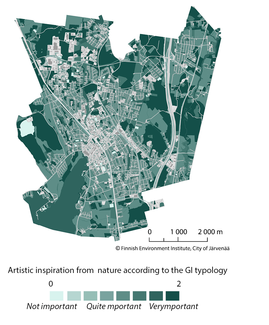
Mapped demand for CES based on scored matrices by individual residents in the City of Jarvenpaa, Finland.
Demand for different types of green and blue environments as a source of CES based on scored matrices by individual residents in the City of Jarvenpaa, Finland.
| CES sub-class / GI type |
Forests
|
Croplands
|
Grasslands
|
Allotments
|
Allotments with huts
|
Urban parks
|
House green
|
Green buffer zones
|
Mires and wetlands
|
Lakes
|
Rivers
|
Creeks
|
| Recreation in nature | 2.0 | 0.8 | 1.4 | 0.8 | 0.6 | 1.9 | 1.9 | 1.3 | 1.3 | 2.0 | 1.8 | 1.1 |
| Nature as a subject matter and site for education | 1.9 | 1.3 | 1.9 | 1.0 | 1.0 | 1.5 | 1.5 | 1.4 | 1.6 | 1.8 | 1.8 | 1.5 |
| Natural aesthetics | 1.9 | 1.3 | 1.9 | 1.1 | 1.3 | 1.8 | 1.8 | 1.5 | 1.6 | 2.0 | 1.9 | 1.8 |
| Artistic inspiration from nature | 1.9 | 1.4 | 1.6 | 0.6 | 0.7 | 1.7 | 1.4 | 1.1 | 1.4 | 1.7 | 1.7 | 1.6 |
| Identity value of nature | 1.7 | 1.0 | 1.4 | 0.7 | 0.4 | 1.7 | 1.6 | 0.7 | 0.8 | 1.7 | 1.4 | 1.3 |
| Place for obtaining empowerment from nature | 2.0 | 0.9 | 1.3 | 0.7 | 0.4 | 1.6 | 1.6 | 0.7 | 1.0 | 1.9 | 1.6 | 1.3 |
| Feeling of holiness in nature | 1.7 | 0.7 | 1.1 | 0.1 | 0.3 | 1.0 | 1.0 | 0.6 | 0.9 | 1.3 | 1.3 | 0.9 |
| Intrinsic and bequest values of nature | 1.7 | 1.0 | 1.1 | 0.8 | 0.7 | 1.6 | 1.3 | 0.7 | 1.7 | 2.0 | 2.0 | 1.6 |
| All CES together | 1.8 | 1.0 | 1.4 | 0.8 | 0.7 | 1.5 | 1.6 | 1.0 | 1.3 | 1.7 | 1.6 | 1.3 |
When simple matrix-based maps are used, the restrictions of the method must be kept in mind. The demand map, such as in the given example, reflects the perceptions of people in a given location and they are seldom transferrable to other locations. They are also coarse generalisations and, in reality, there can be several factors that either improve or diminish the demand for certain locations even if the type of environment is important in general. For example, a forest may be located next to an industry with problematic emissions or the quality of water in a certain lake is poor and even aesthetically unpleasing.
Photo series analysis
There is limited access to spatially explicit data in relation to cultural activities. Yet, there is a growing need for territorial planning to incorporate the perception of numbers of visitors who could be attracted by landscape aesthetic or cultural heritage amongst other key cultural values. As representative field data are expensive and time consuming to gather, gaining understanding on how CES can be spatially defined and visualised is still challenging. A novel way to overcome this is to use crowdsourcing information.
Until recently, user generated contents are providing volunteered geographic information in different place-based applications. The very fast rate of image uploading on popular social media platforms offers potential for a new mapping paradigm based on a crowd of observers. Recent studies have used geo-located photographs retrieved from online platforms to explore place perception. Public image storage analysis has already been applied in studies for assessing CES. These studies suggest an empirical approach based on the location of visitors, assuming that visitors are attracted by the location where they take photographs. This approach opens up opportunities to directly analyse the presence of beneficiaries on the provision site which provides a proxy for actual service provision.
The main limitation of using public image storage analysis to retrieve geo-located information is given by the representativeness of the social media platforms or in relation to specific groups. However, the taken photographs can be considered as observed people's preferences which are less vague than declared preferences. The spatial distribution of visitors' preferences provides an indicator of CES, allowing a local analysis of service providing areas and addressing the lack of quantitative indicators of CES. Application Programming Interfaces (APIs) are publicly available for Web 2.0 applications, such as Flickr and Panoramio, allowing accessing the data, including the photograph's metadata, tags and geographic position.
Different spatial analysis methods can be applied to analyse the specific patterns and identify the landscape settings which shape the actual service provision. A systematic visual analytic process, based on expert knowledge, also allows the identification of different CES categories and their relative importance (Figure
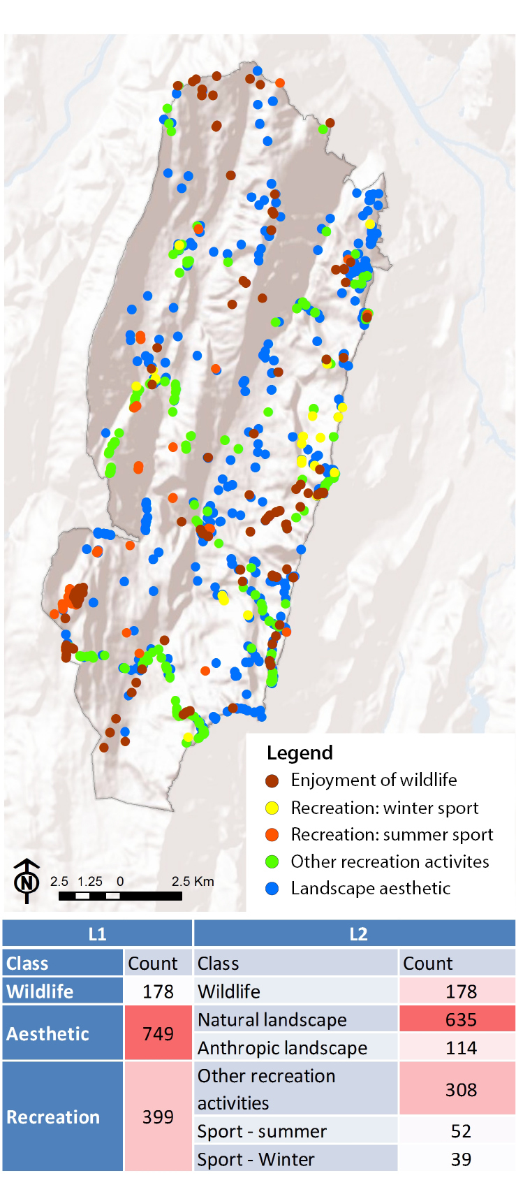
Photo location and count by CES category in Quatre Montagnes Region as case study demonstration (French Alpine Mountain Range).
Moreover, the temporal attributes of the photo-series (date), available on most public photo-archives, can be used to analyse the seasonality of CES (Figure
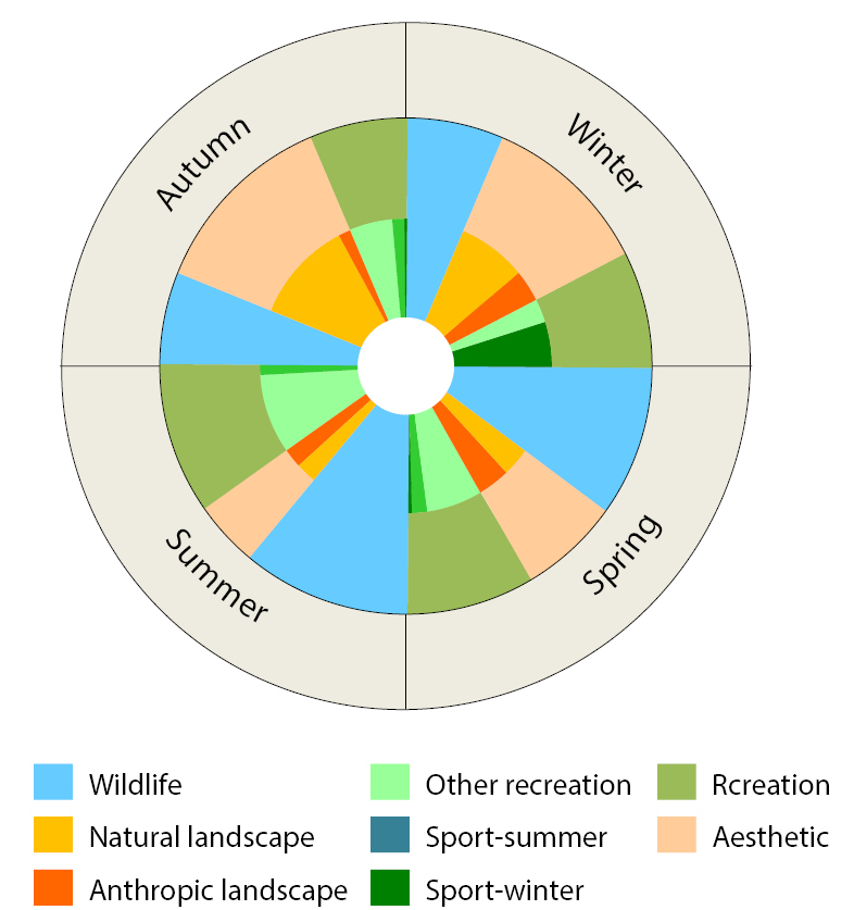
The photo-series analysis can be applied at different spatial scales, ranging from municipality to national, according to the context, photo-density and positional accuracy of the photographs. The final service provision map can therefore inform stakeholders and policy makers at different institutional levels on priority areas (Figure
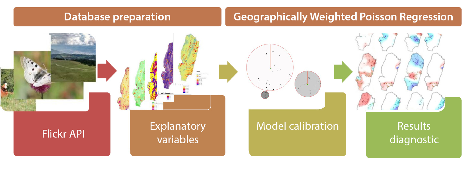
Methodological framework for exploratory analysis of CES through Geographically Weighted Regression (GWR). Given the high diversity of habitats and ecosystems in the study site of Quatre Montagnes, we assume that CES delivery is context-specific and we expect a significant geographical variation in the relations between the photo-count and explanatory variables. The variables correspond to the physical (environmental settings) and infrastructure (opportunity settings) characteristics of the landscape whose spatial variation may affect the CES provision. The spatially weighted regression showed that specific variables correspond to prominent drivers of CES at the local scale. Dominant habitat, accessibility, diversity of habitat and proximity to view points were identified as the variables having a major impact on CES.
Mapping landscape aesthetic service through viewshed analysis
The aesthetic value of landscapes, such as scenic beauty, represents a specific category of CES which has received growing attention in the socio-ecological research. Although the visual aesthetic quality of landscapes has been researched for centuries, standardised and quantitative assessment approaches are so far scarce.
Geo-tagged photographs uploaded on online photo-sharing platforms can be used to locate aesthetically attractive areas and derive the frequentation rate. Together with the biophysical and built-up characteristics of the landscape, the photo-series allows the analysis of complex visual landscapes which are associated with scenic beauty as it is perceived by beneficiaries at specific locations. In open areas, as scenic beauty is especially related to panoramic view, photographs capturing panoramas can therefore be used as spatially explicit data of actual service provision. These data can be related with biophysical factors of the landscapes seen from the respective viewpoints. The visible area and the respective visual indicators can be calculated for each theoretic viewshed, derived from a Digital Elevation Model, corresponding to the photograph location. The viewshed is thus considered as a Service Providing Area from the perspective of the beneficiary (Chapter 5.2). The landscape aesthetic theory allows the linking of landscape visual indicators to the landscape's visual characteristics. Those indicators represent the landscape structures related to the information functions of the landscape which contribute to enjoyment of scenery as a final service. A quantitative framework can thus be applied to identify the landscape variables contributing to the visual landscape attraction.
The procedure for capturing and mapping the visual character of the landscape has been applied in the same study region as the photo series analysis (Figure
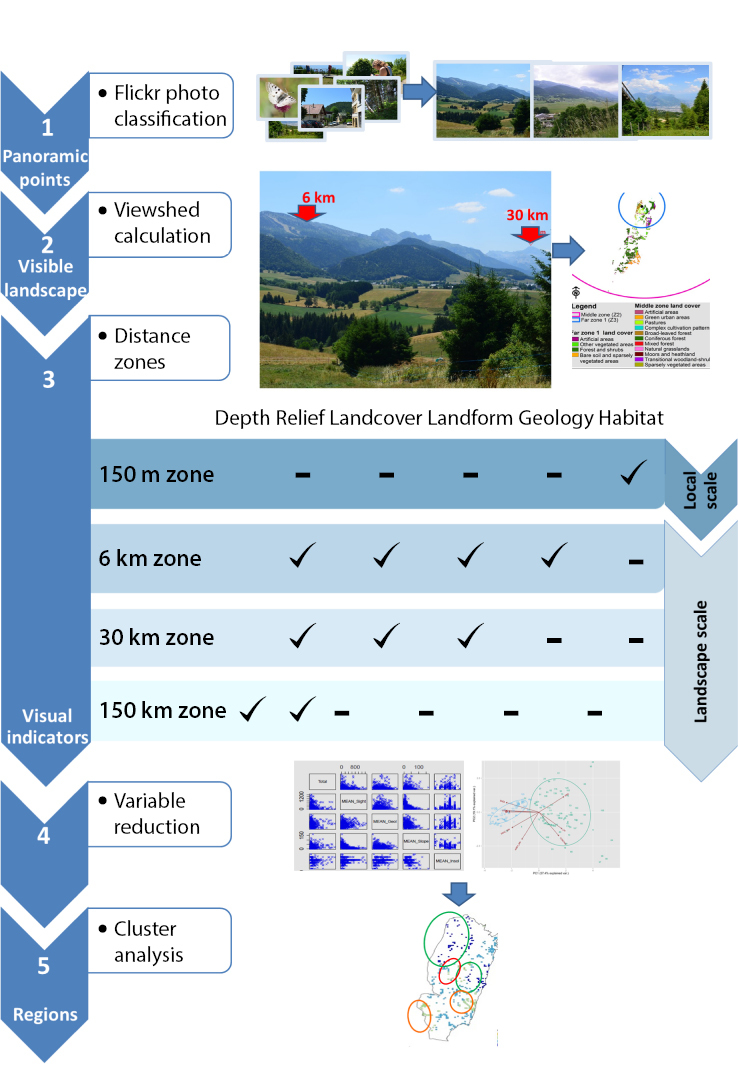
Methodological framework for visual landscape assessment. The visible area (viewshed) was calculated for each location of photo representing panoramic views. The four distance zones were set to respect the degrading visual properties with increasing distance from the viewpoint.
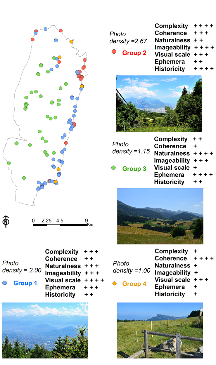
Landscape clusters based on the visual indicators. Four different typologies of landscapes - corresponding to groups of viewsheds - emerged as distinct clusters. The spatial distribution of the landscape groups showed a clustered pattern, allowing a regionalisation of the landscape characters.
This approach provides a framework for performing a systematic analysis of scenic beauty aspects and facilitates interpretation of the landscape information function. By expressing the actual service provision in a spatially explicit way, we can learn about the beneficiaries' perception and the landscape's visual character providing integrated information which can support landscape monitoring and regional planning.
Modelling CES supply using the opportunity spectrum approach: ESTIMAP recreation
Public, nature-based, outdoor recreational activities include a wide variety of practices ranging from walking, jogging or running in the closest green urban area or at the river/lake/sea shore, bike riding in nature after work, picnicking, observing flora and fauna, organising daily trips to enjoy the surrounding beauty of the landscape, amongst a myriad of other possibilities. These activities have important roles in human well-being and health. While tourism is an occasional activity, local outdoor recreation affects the daily life of people. The ESTIMAP recreation model (see also chapter 4.4) assesses the capacity of ecosystems to provide nature-based outdoor recreational opportunities which can be enjoyed on a daily basis. The model consists of three parts: (1) Recreation Potential (RP); (2) Recreation Opportunity Spectrum (ROS); (3) The number of potential trips.
The Recreation Potential (RP) (Figure
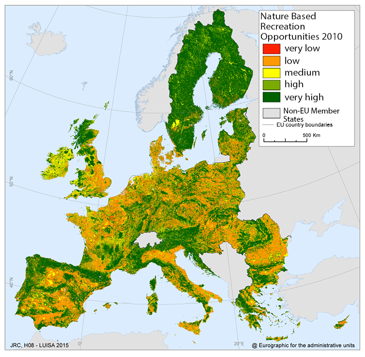
The Recreation Opportunity Spectrum (ROS). People can benefit from the opportunities provided by nature for recreational activities if they are able to reach them. The ROS was chosen as a method to map different degrees of service available according to their proximity to the people. First, a proximity map is computed by combining Euclidean distance from urban and Euclidean distance from roads. A final map of recreation opportunities is then computed by a cross tabulation between the RP and the Proximity using a second set of parameters with thresholds for the degree of recreation opportunities provided by nature and the degree of proximity and remoteness. Parameters can be based on national standards or law (normative) or on observed data.
Number of potential trips
The potential flow of the service to visitors can be estimated by computing the share of potential trips that can theoretically be undertaken in order to reach the different ROS zones. As mentioned above, the present model addresses daily recreation therefore, according to literature, two reference distances were identified for close-to-home and daily maximum travelled distance: 8 and 80 km.
A moving window with a kernel file is applied to a raster grid of population density to compute an estimate of potential trips per each pixel in the grid per day. Figure
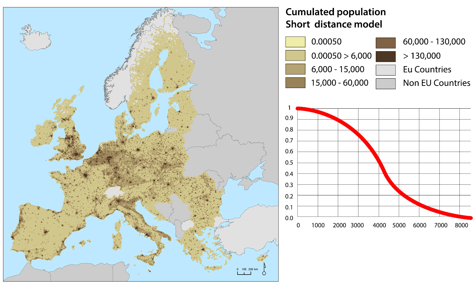
Potential close-to-home trips in Europe. The graph represents the shape of a distance decay function which can be used to model the close-to-home trips. Y axis represents the decay function, X axis the distance.
The percentage of potential trips per ROS zone can be calculated by dividing the sum of potential trips per ROS zone by the total of all possible trips, see graphs in Figure
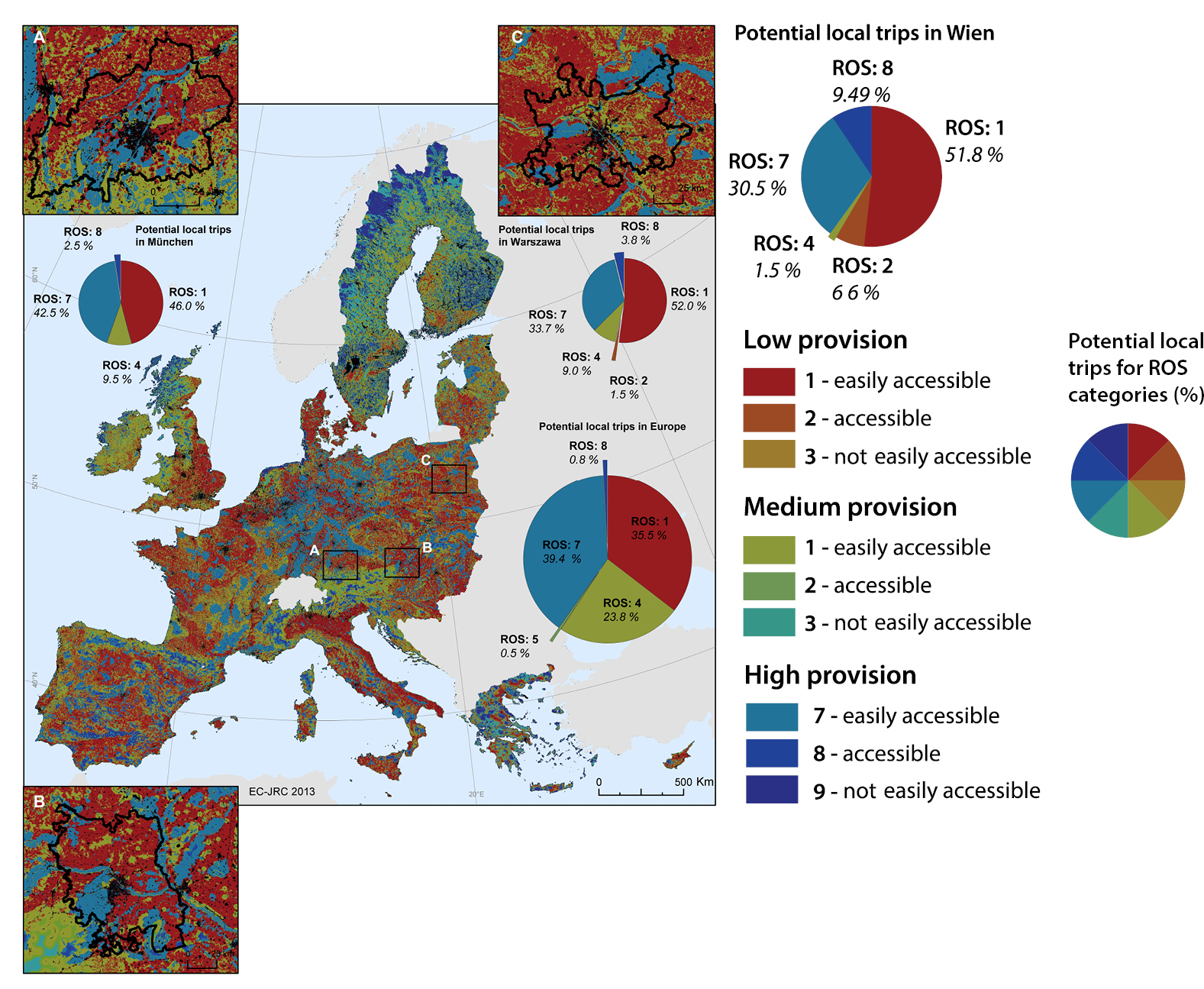
Conclusions
The intangible CES are extremely important for people's well-being in many ways. Mapping them might seem difficult but it is worth the effort. Knowledge of CES capacity, demand and the flow from service providing areas to beneficiaries is crucial in spatial planning, nature tourism development and sustaining and enhancing, for example, people's physical, mental and social health. CES can frequently be overlooked if they are not analysed and visualised in a spatially-explicit way. Mapping provides a means to bring them into discussion along with more easily understood provisioning and regulating services.
Further reading
- Casalegno S, Inger R, DeSilvey C, Gaston KJ (2013) Spatial co-variance between aesthetic value & other ecosystem services. PLOS ONE 8 (6): e68437.
- Di Minin E, Tenkanen H, Toivonen T (2015) Prospects and challenges for social media data in conservation science. Frontiers in Environmental Science 3: 63. doi: 10.3389/fenvs.2015.00063.
- Kopperoinen L, Viinikka A, Zulian G, Yli-Pelkonen V, Niemela J (2016) Developing cultural ecosystem service mapping for spatial planning purposes - Sibbesborg, Finland, as a case study. Ecosystem Services (in review).
- Martinez Pastur G, Peri PL, Lencinas MV, Garcia-Llorente M, Martin-Lopez B (2015) Spatial patterns of cultural ecosystem services provision in Southern Patagonia. Landscape Ecology 31: 383-399.
- Ode A, Tveit MS, Fry G (2008) Capturing Landscape Visual Character Using Indicators: Touching Base with Landscape Aesthetic Theory. Landscape Research 33: 89-117.
- Paracchini ML, Zulian G, Kopperoinen L, Maes J, Schagner JP, Termansen M, Bidoglio G (2014) Mapping cultural ecosystem services: A framework to assess the potential for outdoor recreation across the EU. Ecological Indicators 45: 371-385. http://doi.org/10.1016/j.ecolind.2014.04.018.
- Richards DR, Friess DA (2015) A rapid indicator of cultural ecosystem service usage at a fine spatial scale: content analysis of social media photographs. Ecological Indicators 53: 187-195.
- Schirpke U, Tasser E, Tappeiner U (2013) Predicting scenic beauty of mountain regions. Landsc Urban Plan 111: 1-12.
- Tenerelli P, Demsar U, Luque S (2016) Crowdsourcing indicators for cultural ecosystem services: A geographically weighted approach for mountain landscapes. Ecological Indicators 64: 237-248.
- Tenerelli P, Puffel C, Luque S (2016) Spatial assessment of aesthetic services in Alpine region: combining visual landscape with Volunteered Geographic Information. Landscape Ecology (in review).
- Zulian G, Paracchini ML, Maes J, Liquete Garcia MDC (2013) ESTIMAP: Ecosystem services mapping at European scale. (E. U. R.-S. and T. R. Reports, Ed.). European Commission. Retrieved from http://publications.jrc.ec.europa.eu/repository/bitstream/111111111/30410/1/lb-na-26474-en-n.pdf.
5.6. Integrative approaches
Ecosystem services (ES) are an integrative multi-, inter- and trans-disciplinary field of study per se (see Chapter 2.1). Therefore it is necessary to integrate multiple approaches, methods and data of varying quality and quantity (see Chapters 4 and 5) as well as experts from multiple backgrounds (see Chapter 4.6) in ES mapping and assessment projects. Depending on the purpose of the map product, the most suitable methods and available data need to be chosen and integrated accordingly (see Chapter 5.4).
Integration takes place on different spheres such as different ES (regulating, provisioning, cultural) spatial and temporal scales, domains, (biophysical, social, economic), methods and data (e.g. direct measurements, modelling, interviews) and levels of application (i.e. global, national, regional or local decision- making). The enormous complexity of ES maps and the processes of producing them require a broad range of approaches - from rather simple to complex - that can be integrated in order to harness the advantages of each and to deliver the most applicable and reliable results. However, a more complex approach does not always deliver more robust or more applicable outcomes. For some applications, less can actually be more (or at least sufficient) as was previously stated in the 14th century: "It is futile to do with more things than which can be done with fewer" (cf. Occam's Razor and Chapter 5.4).
The following four sub-chapters introduce different integrative ES mapping and assessment approaches. All approaches can be applied in combination with the concepts and methods described in the preceding chapters.
The tiered ES mapping approach (see Chapter 5.6.1) provides a suitable conceptual framework to combine different levels of complexity from tier 1 to tier 3. Participatory GIS (PGIS; Chapter 5.6.2) is another highly integrative approach combining various kinds of knowledge perspectives with spatial information in a straightforward manner. Harnessing citizens' knowledge and willingness to voluntarily contribute to data gathering is the idea of citizen science as described in Chapter 5.6.3. The ES 'matrix' (see Chapter 5.6.4) is based on spreadsheets that link geospatial units to ES supply or demand providing relatively quick outputs in a spatially explicit manner.
Further reading
- Burkhard B, Kroll F, Nedkov S, Muller F (2012) Mapping supply, demand and budgets of ecosystem services. Ecological Indicators 21: 17-29.
- Maes J, Crossman ND, Burkhard B (2016) Mapping ecosystem services. In: Potschin M, Haines-Young R, Fish R, Turner RK (Eds.) Routledge Handbook of Ecosystem Services. Routledge, London, 188-204.
5.6.1. A tiered approach for ecosystem services mapping
Introduction: The need for a tiered approach in ES mapping
Understanding strengths and weaknesses of the different ecosystem services (ES) mapping methods is crucial for understanding what information can be derived from a map and how applicable it eventually will be. Particularly, information about reliability, accuracy and precision of ES maps is important for users to determine their suitability in a specific context (see Chapters 3.7 and 6.3). ES mapping approaches can broadly be classified into five categories:
A simple and widely used approach directly links ES to geographic information, mostly land cover data and is often referred to as the "lookup table" approach. The land cover data are used as proxies for the supply of (or demand for) different ES. The ES in the lookup table can be derived from statistics such as crop yield for agricultural production.
Approaches, mainly relying on expert knowledge (see Chapter 4.6), include expert estimates of ES values in lookup tables but also other methods such as Delphi surveys.
The "causal relationship" approach estimates ES based on well-known relationships between ES and spatial information retrieved from literature or statistics. For example, timber production can be estimated using harvesting statistics for different areas, elevations and forest types provided in a national forest inventory.
Approaches that estimate ES extrapolated from primary data such as field surveys linked to spatial information.
Quantitative regression and socio-ecological system models that combine field data of ES as well as information from literature linked to spatial data.
To provide guidance in the choice of the appropriate ES mapping method and to enhance comparability between different ES assessments, tiered approaches can be used. The methods can be categorised into tiers with increasing complexity between the different levels such as, for example, in the TEEB (The Economics of Ecosystems and Biodiversity; http://www.teebweb.org/) tiered approach. This idea has also been implemented in the InVEST model (see Chapter 4.4) where a simple (tier 1) and more complex (tier 2) approach is suggested.
Usually the tier 1 approach relies on widely available data and the tier 2 approach includes more specific information for the case study area. Another well-established example is the IPCC tiered approach which structures and facilitates the reporting on climate change at global and national scales. Inventory reports on national greenhouse gas refer to different tiers when describing the methods used and changes in methods from one report to another are related to the tiers defined.
A tiered approach for ecosystem services mapping
Similar to the approaches mentioned above, a tiered approach for ES mapping is proposed in this chapter: it is most useful to define the tiers according to the goal of the mapping exercise (see Chapter 5.4) to make sure the information relevant for the related decision-making process is provided. This supports the efficiency of the mapping process avoiding far too complex approaches where rough estimates would be sufficient.
In a first step, the different components of the analysed human-environment system should be described which include the ecosystems and ES as well as the beneficiaries and institutions involved and their interactions. For example, for microclimate regulation in urban areas, the considered ecosystems are usually green urban areas, the service they provide is microclimate regulation, beneficiaries are residents and institutions are city planning agencies. These system components can be described at different levels of detail, for example, the ecosystem can be described in terms of its condition and structure (see Chapter 3.5), the service provided can be quantified in different units (see Chapter 2.4), the ES demand can be structured according to different beneficiary groups (Chapter 5.1) and different instruments of institutions including NGOs or businesses (see Chapter 7), for example, can be identified. This description of components should make the boundary of the considered system and the spatial and temporal scale explicit. ES beneficiaries and institutions represent relevant stakeholders who could be considered in the decision-making process.
Once these components have been described, the appropriate tier and associated ES mapping method can be selected. To guide this selection, we present a decision tree in Figure
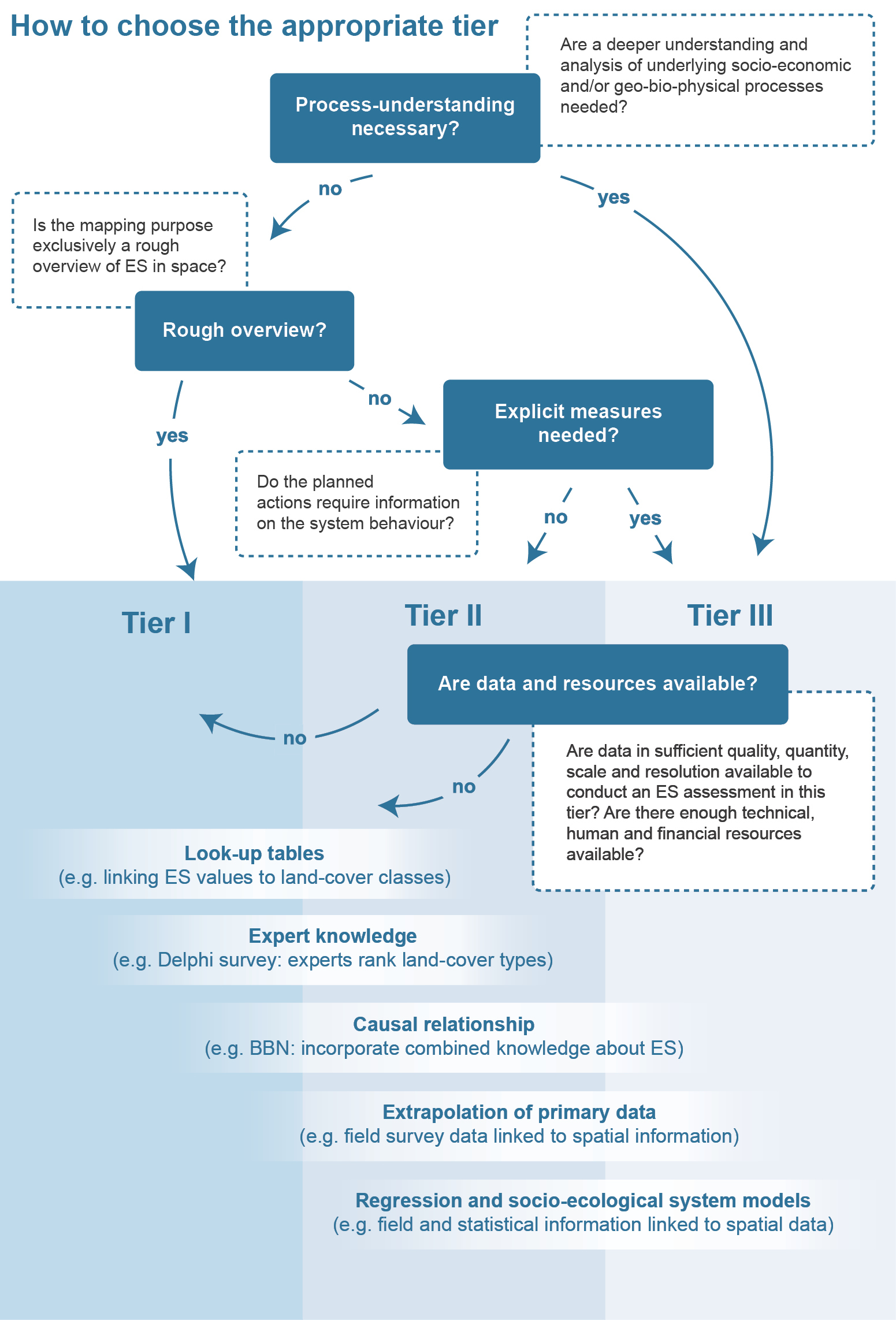
We associated the five different categories of ES mapping methods (see above) with the different tier levels: while most methods are applicable at all tier levels, they usually have a focus at a certain level as indicated in Figure
In this example, we illustrate the tiered approach for mapping microclimate regulation within urban areas with ES mainly provided by green space and important in the context of heat island effects. The components of the human-environment system include green urban spaces as ecosystems, microclimate regulation as provided ES, residents as the main user group and city planning agencies as main institutions. If the purpose is to provide a rough overview, i.e. to compare cities or city districts, no detailed process-understanding is required and a tier 1 approach would be most suitable. Using a lookup table approach, the microclimate regulation can be estimated based on the amount of green space as illustrated in Figure
If the map is to be used to analyse microclimate regulation in more detail without providing information for an explicit management measure targeting system components or processes, a tier 2 approach can be applied. Here, we present a causal relationship approach, where the green volume is estimated by combining high resolution remote sensing data with LU/LC information: Green areas are estimated from the remote sensing information based on the normalised-difference-vegetation-index (NDVI), which allows, for example, identifying single trees. Additionally, the remote sensing data provides information about the height of these identified green areas to estimate the volume. As reducing the urban heat islands by increasing microclimate regulation requires an understanding of how certain measures such as changes in the amount and/or structure of green area quantitatively affect the cooling potential, a process-understanding is needed guiding us to a tier 3 approach.
In a tier 3 approach, the cooling effect is estimated based on a model combining ecological information, i.e. the cooling potential of various vegetation types with the given green infrastructure and their green volumes: the volume of green infrastructure can be derived from a detailed land use typology at the cadastral level based on field surveys with classes such as private yards, sport facilities and infrastructural green. Each class of the typology is related to the amount of trees, grasses, shrubs and settlement or infrastructure present. For the categories tree, grass and shrubs, the volume is estimated based on well-known geometric relations and combined with remote sensing information. The potential cooling effect for high, middle and low green infrastructure can then be modelled considering climate information such as precipitation, temperature and solar radiation. Finally, the effect of infrastructure such as roads or buildings on the cooling potential is considered for estimating the resulting cooling effect.
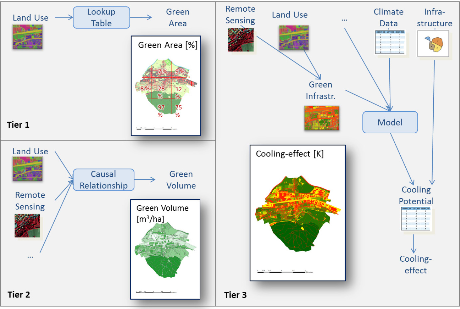
Conclusions
The suggested concept and decision tree provide guidance in the selection of the appropriate tier and associated methods for mapping ES. The presented tiered approach distinguishes the different tiers according to their purpose i.e. the intended use of the ES map. Thus it ensures that ES maps provide information useful to decision-makers in the specific context avoiding either the application of over-complex and resource intensive methods resulting in high costs at a level of complexity of methods which might not be required or over-simplified assessments which could mislead decision-makers.
If we want the concept of ES to be used by decision-makers in the next decades, ES mapping needs to be of high quality and provide precise and reliable information. To provide a solid ground for decision-making, the selection of ES maps should not only be based on methods and data available, but also on the ES that are assessed, because the lack of consideration of relevant ES can significantly change ES trade-off assessments and the selection of alternative policy options.
Further Reading
- Gret-Regamey A, Weibel B, Kienast F, Rabe S-E, Zulian G (2015) A tiered approach for ecosystem services mapping. Ecosystem Services 13: 16-27.
- Martinez-Harms MJ, Balvanera P (2012) Methods for mapping ecosystem service supply: a review. International Journal of Biodiversity Science, Ecosystem Services & Management 8: 17-25.
5.6.2. Participatory GIS approaches for mapping ecosystem services
Introduction
Participatory mapping is the process where individuals contribute to the creation of a map. It can be applied to ecosystem services (ES) assessment by engaging various stakeholders to identify and map a range of ES that originate from location-based knowledge. These approaches are commonly known as Public Participation GIS (PPGIS) or Participatory GIS (PGIS) (in this chapter, the acronym PGIS is used) and refer to the use of spatially explicit methods and technologies for capturing perceptions, knowledge and values of individuals or groups via surveys and/or workshops, with the aim of using this spatial information in land use planning and management processes. PGIS approaches represent a spatially explicit socio-cultural assessment of ES. The location-specific mapping communicates the assigned environmental values, i.e. the judgement regarding the worth of objects such as places, ecosystems and species.
Since the early 2000s, when PGIS approaches addressing community values for ES appeared, this field has increased exponentially for pragmatic and practical reasons such as: the idea of crowd wisdom to create knowledge from the masses, the lack of spatial data in specific contexts or for certain services, the need to include socio-cultural perceptions for ES assessment, technological development allowing sophisticated mapping solutions (e.g. web-based participatory mapping) and the democratic aim of bringing stakeholders to participate in the assessment of the value of nature's services and related decision-making. The increased use of PGIS has resulted in its application in multiple contexts and with different aims including informing land use planning, rural landscape planning, protected area management, conservation planning, urban planning and coastal zone management amongst others.
Collecting data through participatory mapping approaches
Data collection with PGIS approaches represents pluralism. Common data collection methods include self-administered surveys, either web- or paper-based, face-to face surveys and workshops (see Table
Three common data collection approaches in PGIS (web-based surveys, face-to-face surveys and workshops) for ES assessment and their characteristics.
| Characteristics | Web-based surveys | Face-to-face surveys | Workshops |
| Participants type | Often lay public | Lay public and experts | Often experts (e.g. local inhabitants with ecological knowledge, environmental specialists, planning practitioners) |
| Time, cost and facilitation requirements | Time efficient but resources needed for inviting participants, no facilitation needed and participation not restricted by specific time and place | Time consuming as each person needs to be met individually, resources also needed for inviting participants and training interviewers | Time efficient as it allows all data gathering during the workshop, but demanding for preparation and training facilitators |
| Sampling method | Random sampling, volunteered open participation | Random sampling, on site recruitment, meaningful sampling, stakeholder prioritisation | Meaningful sampling, stakeholder prioritisation |
| Sample size and representativeness | Easier to reach a larger and more representative sample, although survey respondent rate often remains low (under 15%) | Depends on available resources, possibility to control representativeness | Remains often low, statistical representativeness not targeted |
| Type of participation and its effect on data quality | Instrumental and self-administered, difficult to analyse the level of understanding of the participant and data quality | Self-administered but allows facilitation and a detailed exploration of the issue analysed, contributes positively to data quality | Allows communication among participants and detailed exploration of the issue analysed (deliberative mapping), contributes positively to data quality |
PGIS mapping of ES involves either digital mapping interfaces, often web-based, with zoomable background maps or printed map layouts commonly presenting one given scale. Information, given on the background maps typically includes aerial/satellite image overlaid with basic map elements, or topographic maps showing, for example, relief and basic natural and man-made features. The most often applied method for marking has been point placement (e.g. movable plastic discs or stickers) followed by drawing polygons presenting areas or using predefined land units as a basis for assigning values.
Most commonly applied typologies for mapping include ES classifications (MA, TEEB, CICES, see Chapter 2.4), adaptations of these to specific contexts or landscape values and landscape services typologies developed in case studies and based on research on social values. Direct ES identification and valuation through an inductive approach, not deriving from a given typology, have been rarely applied.
Analytical process
A wide variety of analytical approaches can be applied to PGIS data on ES (Figure
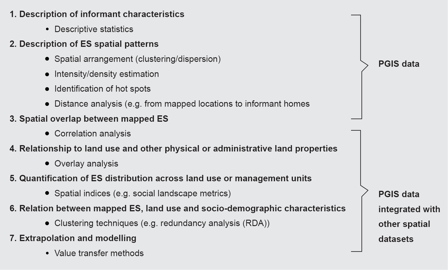
Example of an analytical process for PGIS data from basic descriptive steps to more advanced spatial and statistical analysis where PGIS data is integrated with other spatial data sets.
Spatial concurrence is commonly studied through overlay analysis to explain the relationship to physical land features (such as land cover, land use, management units, land change) or ecological data. In addition, spatial indices such as landscape metrics derived indices are common to quantify the distribution across different land use or management units within the study area. Clustering techniques have been found useful for exploring the potential relation between the mapped ES and, for example, land use and socio-demographic characteristics of informants. Interest has also been paid to extrapolate and model the distribution of the participatory mapped ES to locations where data were not collected through value transfer methods. Analysis of ES bundles has not been frequent but is gaining more attention as is the analysis of ES flows and trade-offs.
Opportunities and challenges for future research and practice
Several case studies show that socio-cultural valuation of ES through PGIS has successfully facilitated the identification of spatial areas of ES supply and demand and how these vary between stakeholder groups. PGIS data may also be integrated with spatial data on ES produced through other methods, advancing trans-discipline and more comprehensive ES assessment. Some opportunities and challenges for PGIS approaches may be identified and formulated around the following three points.
Firstly, PGIS allows addressing certain aspects of ES that cannot be evaluated without participation. PGIS approaches have potential to enhance the appreciation of abstract, symbolic and intrinsic values that landscapes and ecosystems provide to humans. Insufficient acknowledgement of these values has been addressed in literature as one of the recurring critiques of the ES framework. Certain ES categories such as cultural services (e.g. landscape aesthetics, cultural identity, place attachment, etc.), might naturally better fit in PGIS than non-PGIS methods, since PGIS can directly capture the perceptions and values individuals have towards ES. Cultural services are also often inferred from proxy data underestimating the multiple socio-cultural benefits widely recognised as critical for human well-being.
Secondly, new opportunities arise through information technologies (ITs). The mushrooming new ITs and increasingly available open source spatial data sets can facilitate the application of PGIS methods through citizen science (e.g. via smart-phones and use of open source high resolution imagery or topographic maps) opening new possibilities for open public access of ES mapping for decision-making (Chapter 5.6.3). In data-scarce regions, PGIS has also been proposed as an alternative to complex and expensive data-building processes to map ES. In this case, depending on the use of the data, it is important to evaluate the accuracy of information outputs (e.g. to compare participatory mapped ES data with physical landscape features mapped by participants, or with modelling approaches).
Thirdly, it should be emphasised that participation should be in the core of PGIS. Capacity building and social learning should always be seen as important aims of participatory activities. Another important aspect of mapping ES through PGIS is to actually integrate this data into land use planning and decision-making regarding ecosystem protection, conservation and management and to communicate to the participants how it was applied. This would enhance public participation in practice and it would not only be seen as consultation which, unfortunately, is prevalent in the current PGIS practice. Hence, integration of the gathered spatially explicit knowledge into decision-making remains a challenge for the future and requires also significant commitment by researchers and facilitators as well as resources to appreciate PGIS as a process in ES assessment.
Further reading
- Bryan BA, Raymond CM, Crossman ND, Macdonald DH (2010) . Targeting the management of ecosystem services based on social values: Where, what and how? Landscape Urban Planning 97: 111-122.
- Brown G, Fagerholm N (2015) Empirical PPGIS/PGIS mapping of ecosystem services: A review and evaluation. Ecosystem Services 13: 119-133.
- Brown G, Pullar DV (2012) An evaluation of the use of points versus polygons in public participation geographic information systems using quasi-experimental design and Monte Carlo simulation. International Journal of Geographical Information Sciences 26: 231-246.
- Burkhard B, Kroll F, Nedkov S, Muller F (2012) Mapping ecosystem service supply, demand and budgets. Ecological Indicators 21: 17-29.
- Fagerholm N, Kayhko N, Ndumbaro F, Khamis M (2012) Community stakeholders' knowledge in landscape assessments-Mapping indicators for landscape services. Ecological Indicators 18: 421-433.
- Garcia-Nieto AP, Quintas-Soriano C, Garcia-Llorente M, Palomo I, Montes C, Martin-Lopez B (2014) Collaborative mapping of ecosystem services: The role of stakeholders' profiles. Ecosystem Services 13: 141-152.
- Klain SC, Chan KM (2012) Navigating coastal values: participatory mapping of ecosystem services for spatial planning. Ecological Economics 82: 104-113.
- Palomo I, Martin-Lopez B, Potschin M, Haines-Young R, Montes C (2013) National Parks, buffer zones and surrounding lands: mapping ES flows. Ecosystem Services 4: 104-116.
- Raymond CM, Bryan BA, MacDonald DH, Cast A, Strathearn S, Grandgirard A, Kalivas T (2009) Mapping community values for natural capital and ecosystem services. Ecological Economics 68(5): 1301-1315.
- Raymond CM, Kenter JO, Plieninger T, Turner NJ, Alexander KA (2014) Comparing instrumental and deliberative paradigms underpinning the assessment of social values for cultural ESs. Ecological Economics 107: 145-156.
- Sherrouse BC, Semmens DJ, Clement JM (2014) An application of Social Values for ES (SolVES) to three national forests in Colorado and Wyoming. Ecological Indicators 36: 68-79.
5.6.3. Citizen science
What is citizen science
The term "citizen science" (CS) already suggests that citizens somehow are involved in science. Synonyms occasionally used are crowd science or crowd wisdom (with collective intelligence considered superior for solving social or environmental problems).
A citizen, in this context, refers to amateurs or non-scientists voluntarily contributing to or participating in data gathering (such as observations of natural phenomena or species) or in scientific projects. Scientific projects involving citizens are often called participatory research. In many instances, volunteers are collecting, for example, additional biological or astronomical data, with the most popular and well-known citizen science activity probably being bird watching. In other cases, citizens may be more deeply involved in defining research questions and in designing and running the projects in which professional scientists may or may not be involved at all. Such projects may take place in a citizen association focusing on, for example, regional history, language, landscapes.
Nowadays, research is dominated by professionals but only two centuries back, amateur researchers such as Benjamin Franklin or Charles Darwin were more the rule rather than the exception. During the last decades, CS and participatory research have increased tremendously in various fields of science such as astronomy, biology, environmental science, history or the observation of weather phenomena such as cyclones. In recent discussions about the quality of data generated in CS projects, expertise, motivation and honesty of CS contributors have been questioned by scientists.
While data quality criteria usually are available, potential conflicts of interest may be harder to detect and address (see suggested reading at the end of this chapter). What has been shown is that CS may improve decision-making, generate new knowledge and innovations, empower citizens and generate political discourse and concern.
In the context of ecosystem services (ES) mapping, CS implies that public participation can well go beyond participatory monitoring of ES in a research project. For instance, groups of urban gardeners could map their ES use with the objective of identifying their main interests or the diversity of their contributions to food production or their recreational activities.
In the rest of this chapter, we focus on CS contributing to the mapping and assessment of ES and present some of the methods available for CS / participatory approaches.
CS approaches in ES mapping and assessment
Different types of ES can be distinguished (see Chapter 5.5) and different methods and approaches are available to map and assess them (see Chapter 3.2). Many cultural ES are especially difficult to address via scientific mapping and modelling tools not involving the broader public, as cultural ES often depend on the preferences of users which may vary considerably locally or regionally. Excepting touristic activities, for which much visitor or overnight stay data are available, large information deficits still exist about other cultural ES such as gardening, outdoor activities, appreciation of cultural heritage or intellectual experiences which are much more difficult to assess without asking or involving citizens. Thus, in the context of cultural ES, CS projects have a huge potential to increase our knowledge base and contribute to improving decisions and management. Furthermore, citizens increasingly contribute to public debates and decision-making, especially concerning the governance of regulating or provisioning services by, for instance, discussing and defining environmental thresholds such as the use of water resources.
Which methods and tools are available for participatory mapping
In this section, we briefly present four of the participatory mapping methods available for CS in the context of ES mapping and assessment, covering work with conventional paper maps or tables, or digital tools such as geographic information systems (GIS) or smartphone apps. All methods can be used with different levels of citizen and scientist involvement. The higher the level of involvement of citizens, the higher the level of knowledge needed for citizens, for instance, about different ES, to handle spatial data in a geographic information system, to prepare paper or digital maps of the study area, or to evaluate information generated during the CS project.
In every ES mapping approach, citizens and scientists need to define the mapping perspective, i.e. whether they want to address the (potential) supply of, the demand for, or the actual use (= flow) of ES (see Chapter 5.1). Additionally, in most approaches, spatial and temporal units / coverage also need to be clarified (see Chapter 5.7.5).
ES use has been mapped by citizens and scientists using the MapNat smartphone application. Colours of flags indicate different types of ES use. The selected ES use also indicates the frequency of use and the importance, both reflecting the view of the person who mapped the ES use (Figure
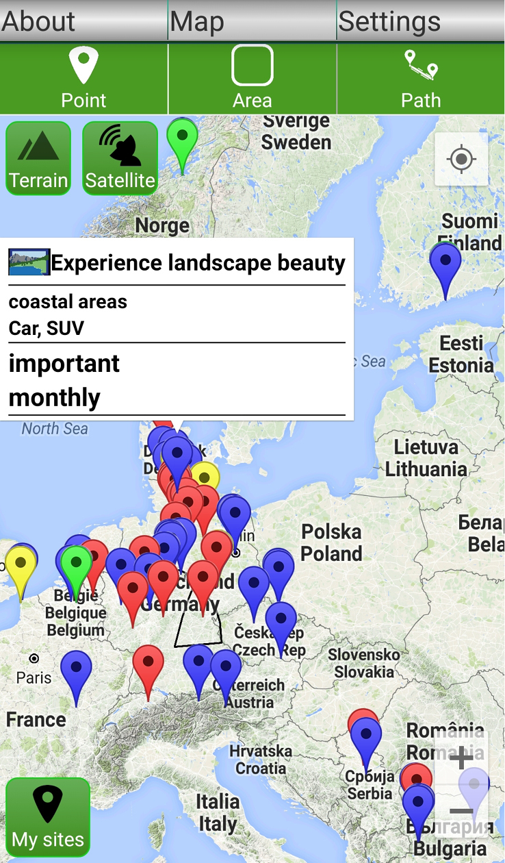
Four CS-compatible mapping examples
Mapping ES with paper maps: Identifying and locating ES on topographic or thematic maps can be carried out as an indoor or an outdoor approach, the latter enabling participants (at least partly) to view and observe the area of interest. Mapping units may be predefined, for example, using units of land cover, or may be identified during the project as, for example, spatial units are assumed to differ between ES. For a quick qualitative ES mapping/assessment (tier 1; see Chapter 5.6.1), one workshop or one field visit may be sufficient, while the generation of more detailed information (tiers 2-3) can be expected to require more time and/or additional sources of information. ES identification and mapping can be carried out individually, either resulting in calculated ES means or ranges or both. Alternatively, ES can be mapped based on a group consensus (called deliberative mapping). The approach can be used to map (potential) supply of and demand for ES, trade-offs, mismatches etc. Data collected with paper maps can be digitised afterwards in GIS (Figures
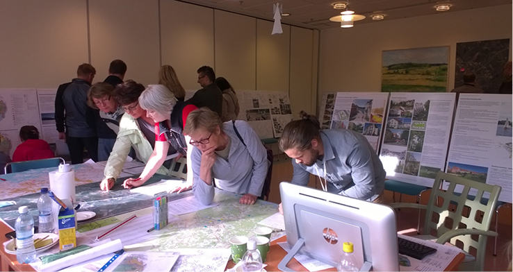
Using paper maps in a local master plan exhibition to collect cultural ES related values, in Sipoo, Finland. Although a digital map of the planning area (see computer in front) was available for citizens, paper maps were preferred by them.
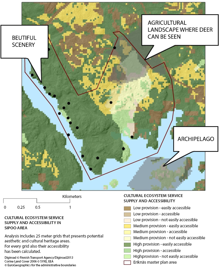
A map presenting the opportunity spectrum of the CES group 'Aesthetics and cultural heritage' in the background and residents' point and polygon markings of the same CES group. Examples of open-ended explanations of the markings have been added on the map. The border of the local master plan area is shown as well.
Mapping ES with GIS: This approach is comparable to the first, the difference being the replacement of paper maps by PCs, laptops or tablet computers (see also PPGIS Chapter 5.6.2). The great advantage of digital mapping is that different types of spatial information can be linked or combined, for example, to derive appropriate mapping units, as well as evaluating ES mapping results. However, at least one citizen or scientist with GIS software experience is needed. The approach can be used to map (potential) supply of and demand for ES. The technical threshold might, however, invoke a selection bias dependent on the knowledge of the involved participant.
The Matrix method to map ES: This method is presented in Chapter 5.6.4. In CS projects, both paper and digital versions may be used. As explained in the previous examples, the matrix method can also be applied individually or as a group exercise and the approach is also suitable for mapping (potential) supply of and demand for ES and, additionally, actual ES use.
Use of a smartphone app such as MapNat for ES mapping: Similar to mapping ES with GIS, MapNat is a participatory GIS approach (see Chapter 5.6.2). Mapping ES uses the GPS (geo-positioning) unit of the smartphone or a tablet to locate ES at the current position of the user. Alternatively, app users can just use their fingers to map ES directly on the device's screen. In this tool, the mapping perspective is focusing on recording the actual use of ES, either directly during ES use, or afterwards identifying the location in the app's map view. This method can also be applied individually or as a group exercise. Contrasting with the previous examples, this tool also provides access to the ES records and valuations of all other app users worldwide (Figure
Further reading
- Bela et al. (2016) Learning and the transformative potential of citizen science. Conservation Biology 00:0, 1-10. doi: 10.1111/cobi.12762
- Dickinson and Bonney (Eds) (2013) Citizen Science: Public Participation in Environmental Research. Cornell University Press, Ithaca & London, 304 pp.
- Editorial (2015) Rise of the citizen scientist. NATURE 524, 265.
CS organisations
Citizen Science Alliance: http://www.citizensciencealliance.org/
European Citizen Science Association: http://www.citizen-science.net/
CS definitions
http://www.openscientist.org/2011/09/finalizing-definition-of-citizen.html
https://en.wikipedia.org/wiki/Citizen_science#Definition
CS platforms
ZOONIVERSE (https://www.zooniverse.org)
Main German platform (in EN and DE): http://www.buergerschaffenwissen.de/en
CS example Cyclones http://www.cyclonecenter.org/#/about
Tools
qGIS: http://www.qgis.org/de/site/index.html
MapNat, ES mapping App: http://www.ufz.de/index.php?en=40618
Harava: https://www.eharava.fi/en/
Maptionnaire: https://maptionnaire.com/en/
5.6.4. Ecosystem services matrix
Introduction
Ecosystem services (ES) are spatio-temporal explicit phenomena. Thus, ES supply, flow and demand (see Chapter 5.1) can be linked to units in space and time. One mapping method is the ES 'matrix' approach, which links ES to appropriate geo-biophysical spatial units. Thereafter, their supply, flow and/or demand are ranked using a relative scale ranging from 0 to 5 (not relevant to very high, see Figure
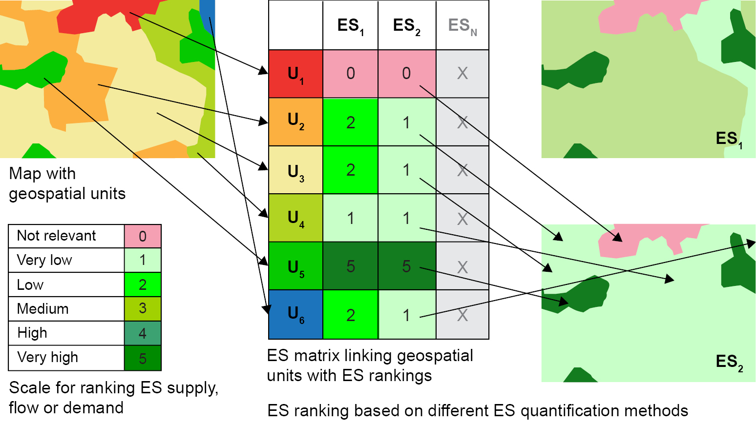
Approach
The ES matrix provides a very flexible ES mapping methodology that can be applied on all spatial and temporal scales (see Chapter 5.7.5), for all ES (see Chapter 2.4), various multidisciplinary ES quantification approaches (see Chapter 4) and for different mapping purposes (see Chapter 5.4).
As shown in Figure
- Selection of ES study area;
- Selection of relevant geo-biophysical spatial units (forming the assessment matrix lines/y-axis);
- Collection of suitable spatial data (e.g. land cover/land use (LULC) data, habitat map, soil map, hydrological map);
- Selection of relevant ES (assessment matrix columns/x-axis);
- Definition of suitable indicators for ES quantification;
- Quantification of ES indicators (using various methods);
- Normalisation of ES indicator values to the relative 0-5 scale;
- Interlinking geospatial units and scaled ES values in the ES matrix;
- Linkage of ES 0-5 rankings to geospatial units to create ES maps; and
- Interpretation, communication and application of resulting ES maps.
Figure
Steps 1-6 are strongly related to the purpose of the ES mapping exercise (see Chapter 5.4) and available mapping capacities (data, methods, time and labour). Relevant stakeholders should be involved in the process as much as possible and when necessary. Steps 7-9 are specific for the ES matrix but also other ES mapping approaches and each step is related to characteristic uncertainties (see below). Step 10 refers to the map-maker to map-user communication (see Chapter 6.4) and applications of ES maps for different purposes (see Chapter 7).
Data sources and quantification methods
In its simplest form of application, the ES matrix assessment uses spatial LULC data as proxies for ES supply. The advantage of LULC data is, besides its availability in many regions of the world, that many provisioning ES (see Chapters 2.4 and 5.5.2) can be specifically and uniquely linked to single LULC types. Timber, for example, is harvested from forests, crops grow on agricultural fields and fish and seafood occur only in water bodies, rivers and the ocean. Regulating ES (see Chapter 5.5.1) and cultural ES (see Chapter 5.5.3) are usually supplied in well-functioning and not too far degraded ecosystems which can be related to more natural LULC types. ES maps, based on LULC information, provide important spatial landscape information which already can be helpful for the identification and awareness-raising of ES and their supply and demand patterns.
In case the ES mapping purpose goes beyond providing a rough overview of ES supply or demand in space, further data and ES quantification approaches can be integrated. The tiered ES mapping approach (see Chapter 5.6.1) helps select the appropriate method based on the mapping purpose, the necessary process-understanding and needed explicit measures and, last but not least, the data and resources availability.
ES data from all three mapping tiers can be integrated into the ES matrix. The use of expert knowledge for ES quantification and qualification has, for example, become very popular and increasingly accepted within the scientific community. More comprehensive ES assessments would otherwise demand large resources in terms of time and personnel. Data from statistics, for instance about agricultural or forestry production or existing studies with relevant information - if available and appropriate - should further be integrated in the ES matrix assessment. Model outcomes provide further useful data applicable for ES mapping (see Chapter 4.4).
In an optimum case, data from all tiers can be acquired for the same area, time and spatial scale and in comparable resolution. These data can then be triangulated in order to be cross-checked and to find the most suitable, reliable and useful (for the specific mapping purpose) ES quantification and mapping method (see also Chapter 4.6). Figure
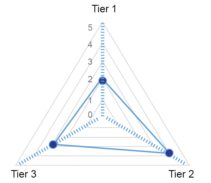
Data normalisation
As mentioned above, the ES matrix approach is based on a normalisation of ES indicator values to a relative scale ranging from 0-5. "0" represents no relevant ES supply or demand. The term "relevant" is mentioned here because "0" does not necessarily mean absolute zero (0.000.....) for all types of ES. It is supposed to reflect the fact that, in natural systems, several ES are constantly supplied, but this supply is not relevant (or not yet perceived to be relevant) for human well-being. At the other end of the scale, "5" represents the maximum ES indicator value. It is important to be clear about what the reference for this maximum value is. In most cases, it is not useful to use global reference values and compare them with regional studies (e.g. using tropical forests' primary productivity as reference for boreal forests). One pragmatic solution is to use only ES indicator values that can be found in the study area, i.e. class 5 represents the maximum amount of ES supplied or demanded in a region.
The data normalisation to the six categories needs to be based on a sound data classification method using appropriate class breaks. Usually the equal intervals (see Chapter 3.3) classification methods should be used to group the data into the 0-5 classes. Outlying values in the maximum value class can be included in the 5-class (i.e. integrating values that are larger than the last equal interval maximum value). In addition, for the lowest values (0-class), a data range smaller than the respective equal interval may be suitable. Classification methods, other than equal intervals such as natural breaks or quantiles, might affect results and are less suitable to make the different classes and their values comparable with each other. Class "4", for instance, intuitively indicates twice as much ES supply or demand than class "2", which also needs to be shown by the data.
The relative data normalisation approach is comparable to the commonly used Likert scale. This scale uses five categories of decreasing (or increasing) values to indicate, for example, frequency (very frequently - frequently - occasionally - rarely - never), agreement, importance or likelihood.
Uncertainties of the ES matrix
The most appealing aspect of the ES matrix approach is perhaps its simplicity of application. The matrix delivers tangible results of ES supply and demand patterns in look-up tables and resulting maps by integrating data from various sources. However, the approach and especially its integrative character include several uncertainties (see also Chapter 6) which are presented in the following, relating to the 10 steps of application shown above:
1. Selection of ES study area
The case study area needs to be representative for the addressed question and region. It needs to reflect the specific local, natural and cultural settings, land management and changing socio-ecological system conditions.
2. Selection of relevant geo-biophysical spatial units
Generalisation (see Chapter 3.2) and categorisation of complex landscapes into a limited number of classes (e.g. LULC types) include simplification and uncertainties. Spatial units are also dependent on spatial data resolution and study area size.
3. Collection of suitable spatial data
Information availability (e.g. appropriate biophysical data on soils, hydrology and vegetation) and data access often limit comprehensive ES studies. In some regions, not all necessary data sets are available (e.g. habitat maps). Further uncertainties can be based on inaccuracies in spatial and thematic data and unsuitability of spatial and temporal scales.
4. Selection of relevant ES
Which ES are really relevant in the case study area and which user groups are benefitting? Are ES imported and exported to/from the region? Especially for data-driven studies, many ES are neglected due to data availability.
5. Definition of suitable indicators for ES quantification
ES indicators need to be robust, scalable and sensitive to changes. Furthermore, appropriate indicator-indicandum (i.e. the subject to be indicated) relations need to be identified and defined. Various indicators are needed for ES trade-off and synergy assessments.
6. Quantification of ES indicators
Uncertainties can be due to the lack of appropriate data for ES quantifications and the use of surrogate indicators, model, measurement and statistical data uncertainties, mismatches between geo-biophysical data and statistical data spatial units or limited knowledge about complex ecosystem functions.
7. Normalisation of ES indicator values
Comparability of data from different sources, varying quality and quantity and across various ES categories is not always given. Moreover, subjectivity in the scoring procedures and data classification include uncertainties.
8. Interlinking geospatial units and ES in the ES matrix
The averaging of ES data over space and time is difficult (a weighting system could help but would complicate communication of results). Usually, ES supply takes place spatially and heterogeneously and aggregation of data, models and indicators without losing relevant information is not easy.
9. Linkage of ES 0-5 rankings to geospatial units
Mismatches of selected spatial units and ES (e.g. difficulties in allocating cultural ES to land cover data), including definition of appropriate service providing areas (see SPA; Chapter 5.2) and ES flows can lead to uncertainties of ES maps. Limited knowledge about complex socio-ecological system linkages, data extrapolation to different or larger regions, the proper representation of multiple ES (2D maps usually only allow the presentation of one ES or ES averages/sums) and GIS software/data issues also add further uncertainties.
10. Interpretation, communication and application of resulting ES maps
Badly designed maps and insufficient end-user interfaces might cause interpretation problems (see Chapter 6.4). Data and map misinterpretation can also be due to lacking knowledge of the study area or general lack of expert knowledge, for example, concerning interactions between landscape management and ES supply. ES information is often too complex and too aggregated for easy and fast understanding. Model and map validation (see Chapter 6.3) and respective uncertainty or reliability measures are, in most cases, not provided with the ES map.
Conclusions
The ES matrix approach has become a very popular methodology for ES mapping. Combined with the tiered approach, various data and ES quantification methods can be used and integrated. The key advantage is the high flexibility and applicability of the ES matrix at various levels of complexity. Less complex applications relatively quickly deliver results that, for example, are useful for awareness-raising or first ES screening studies. The ES matrix is currently applied in several case studies on different spatial scales all over the world and for different mapping purposes. The methodology is increasingly improved by this approach, until the full potential eventually can be harnessed.
Further reading
- Burkhard B, Kroll F, Muller F (2009) Landscapes' capacities to provide ecosystem services - a concept for land-cover based assessments. Landscape Online 15: 1-22.
- Burkhard B, Kroll F, Nedkov S, Muller F (2012) Mapping supply, demand and budgets of ecosystem services. Ecological Indicators 21: 17-29.
- Burkhard B, Kandziora M, Hou Y (2014) Ecosystem Service Potentials, Flows and Demands - Concepts for Spatial Localisation, Indication and Quantification. Landscape Online 34: 1-32
- European Commission Science for Environment Policy (2015) Ecosystem Services and the Environment. In-depth Report 11 produced for the European Commission, DG Environment by the Science Communication Unit, UWE, Bristol. Available at: http://ec.europa.eu/science-environment-policy.
- Hou Y, Burkhard B, Muller F (2013) Uncertainties in landscape analysis and ecosystem service assessment. Journal of Environmental Management 127: 117-131.
- Jacobs S, Burkhard B, Van Daele T, Staes J, Schneiders A (2015) The Matrix Reloaded: A review of expert knowledge use for mapping ecosystem services. Ecological Modelling 295: 21-30.
- Kandziora M, Burkhard B, Muller F (2013) Mapping provisioning ecosystem services at the local scale using data of varying spatial and temporal resolution. Ecosystem Services 4: 47-59.
- Sohel SI, Mukul SA, Burkhard B (2015) Landscape's capacities to supply ecosystem services in Bangladesh: A mapping assessment for Lawachara National Park. Ecosystem Services 12: 128-135.
- Stoll S, Frenzel M, Burkhard B, Adamescu M, Augustaitis A, Bae?ler C, Bonet Garcia FJ, Cazacu C, Cosor GL, Diaz-Delgado R, Carranza ML, Grandin U, Haase P, Hamalainen H, Loke R, Muller J, Stanisci A, Staszewski T, Muller F (2015) Assessment of spatial ecosystem integrity and service gradients across Europe using the LTER Europe network. Ecological Modelling 295: 75-87.
5.7. Mapping ecosystem services on different scales
Mapping of ecosystem services (ES) is inherently related to the topic of scales. Various scale aspects need to be taken into account in order to consider key aspects which are driving decisions in the context of land use management. First of all, the spatial scale is of importance. It is crucial to identify the appropriate spatial scale which refers to the structures, processes, functions and services which are provided or demanded in a spatial unit. This unit might have a local, regional, national, continental, or global extent. Additionally, spatial scale is characterised by the "grain", i.e. the spatial resolution of a map. The higher the spatial resolution (and the smaller the Minimum Mapping Unit, MMU), the more detailed statements may be derived from a map.
Once the spatial scale is clear, the crucial information for successful application of the ES concept is provided by the map content. The thematic resolution of maps should reflect the subject of interest. For some basic statements, for example on soil sealing, the distinction of two thematic classes, sealed and un-sealed, can be sufficient. When it comes to the mapping of more complex processes, functions or services, higher thematic resolution would be required. This is especially true for highly specialised systems. To distinguish the erosion potential of specific crop rotation types, for example, numerous thematic classes are required which reflect the number of crops, the length of a rotation period, the soil management type etc.
The spatial scale, however, should not only refer to grain and extent. The third dimension should also be considered. Slope inclination, relief intensity and the elevation above sea level significantly affect the quantity, quality and distribution of ES.
Mapping of ES at a specific spatial scale reveals insights of the current situation. For the application of the ES concept in policy making or spatial planning, the monitoring of changes, as well as visualisation and evaluation of possible futures is of great importance. Not only spatial "hot spots" and "cold spots" of ES supply and demand need to be considered (see Chapter 5.2), but also "hot moments" and "cold moments" (see Chapters 5.3 and 5.7.5).
Temporal scales range from short-term, seasonal, annual, medium-term, to long-term considerations. Again, depending on the subject and the purpose of a study, the appropriate scale needs to be identified. Cross-sectoral, integrated spatial planning (see Chapter 7.2) at the regional scale, for example, typically refers to the medium term perspective (10 to 20 years in the future). In contrast, sectoral forestry planning (see Chapter 7.3.3) requires both operational short-term planning and long-term consideration of a couple of hundred years to reflect the forest development from planting to final harvesting (see Chapter 5.7.5). Looking backwards, maps of land use changes can reveal insights of past developments which are fundamental for the estimation of future trends in a region's development.
These various dimensions of scale are interlinked. Usually, global considerations take large-scale and long-term topics at lower thematic resolution into account (see Chapter 5.7.3). On the other hand, local or regional studies typically are characterised by deeper understanding of processes and functions and availability of high resolution data regarding spatial and temporal scale (see Chapter 5.7.1). One of the major challenges is the up-scaling of local knowledge on higher scales (see Chapter 3.7). Without the understanding of local structures and processes, the regional, national and global mapping and assessment of ES would run the risk of neglecting essential information which determines the ES performance. Chapter 5.7 gives an overview of different scales of ES mapping, covering regional, national and global perspectives. Marine areas and the interactions of spatial, thematic and temporal scales are specifically addressed.
Further reading
- Reid WV, Berkes F, Wilbanks T, Capistrano D (Eds.) (2006) Bridging scales and knowledge systems: concepts and applications in ecosystem assessment / Millennium Ecosystem Assessment. Island Press/World Resources Institute, Washington, DC.
5.7.1. Regional ecosystem service mapping approaches
Introduction
Human activities and therefore ecosystem services (ES) act on different scales - not only temporally but also spatially. Consideration of these different spatial scales is especially important for a meaningful and precise mapping of ES (see Chapter 5.7). Results can be very different depending on the investigated ecosystem service(s) and the available data sets.
The first barrier is the fact that no clear definition exists about what regional or local mapping approaches mean or include. Most often the area that is mapped is considered as the spatial scale. However, the applied data sets also have different resolutions regarding the technical or thematic scale (ranging from very fine to very coarse) and have therefore the ability to identify important ES or not.
The aim of this chapter is to give a short overview of some necessary requirements that need to be kept in mind when mapping at local or regional scale.
Spatial scales
Local scale
The term local is mainly connected with a specific (geographic) position. Local scale can range from single farms to villages/communities and to smaller administration units (e.g. municipalities). This depends, of course, on the administrative/political or historical conditions of the case study area. However, small protected areas or specific ES that only act over a very narrowly defined extent (e.g. sacred/holy features of nature such as trees) can also be considered local in mapping approaches. In addition, some ecosystems cover only a limited area; for example, species-rich wetlands. In coastal or marine ecosystems, harbours, steep coasts or reefs are, for example, in a specific location and provide many ES.
Local case studies are particularly suitable for more labour-intensive data compilations and method testing. Many participatory mapping studies and direct stakeholder-involved assessments (e.g. focus group surveys) have been undertaken at the local scale. Beyond that, there are several ES that can sometimes only occur at defined extents; scenic views, for example or wild food such as mushroom picking. Mapping these is best done on the matching scale for a precise result of the human preferences and activities contributing to human well-being.
Data sets must be of high resolution to address the peculiarities of local mapping studies. Applying data that is too coarse (e.g. aggregated land cover or land use) will blur the findings. Data mismatches can have a strong misleading effect on land use management and decision-making. Local case studies are important for many participatory steps including communication and raising awareness for ES. Decisions on ecosystem management need to meet local requirements and fine resolution data and information.
Regional scale
A region is an area of indefinite size that is different to the adjacent areas. It can range from a part of a country (e.g. Northern Germany) to a part of the globe (e.g. Scandinavia). This means the term can act as an administrative unit or describe an area based on similar characteristics (e.g. subarctic regions with similar climatic conditions or the Amazon basin). Therefore, regions contain either similar natural or cultural/economic characteristics. Due to the similar features within a region, this spatial scale is a suitable mapping unit for many ES.
In addition, there are specific connotations, such as a tourism region (e.g. the Alps, the Baltic Sea) or a region is important or known for its specific features (e.g. the breadbasket of a country like the Great Plains of the US). Based on these different criteria, regions can also overlap with each other or certain areas within a region could be excluded if they do not possess the functional or homogenous criteria. The term is also very specifically used in some languages, fostering further challenges in the assessment and mapping of ES by delineating case study areas.
In many cases, several data sets are available in aggregated format ranging over a great extent. Land cover or land use data sets can act as an appropriate (first) approach for mapping regional ES (see Chapter 5.6.4).
Mapping methods and data requirements
Local mapping approaches can be quickly supported by direct (participatory) mapping and data acquisition/measuring or ground-truth checks when applying available data sets or other methods. Specific data sets, such as detailed habitat or biotope maps, are available on local scales with high resolution. Supply and demand budgets can be accounted for and mapped more easily. Additionally, web or smart phone based data acquisition (e.g. citizen science; Chapter 5.6.3) are suitable for smaller case studies and stakeholder consultations (interviews, workshops). There are also models that work on the site scale or farm scale, especially for regulating and provisioning services. On the other hand, statistical data are often not available at high resolution information levels due to privacy protection or highly time-consuming acquisition.
Regional mapping approaches contain all available methods (see Chapters 4 and 5). Single indicators, statistical data and modelling can be applied together with stakeholder assessments (e.g. expert interviews). Spatial data resolutions are often > 100 m.
Cultural ecosystem services
Many cultural ES can best be mapped on local or regional scale, allowing the inclusion of specific aspects of preferences and activities. Accessibility is an important point for recreation and tourism, as well as for landscape aesthetics. Points of interest, hiking paths, roads, streams and other landscape features must be included for a comprehensive analysis. In regional maps, aggregated information (for instance, different beach types) is needed to give a more general overview of cultural ES.
Surveys in tourist locations are most often undertaken for a specific purpose to understand the motivation of tourists for visiting a certain place (e.g. beach vs. cultural attractions).
Regulating services
Many of the underlying natural processes included in regulating services are not restricted to small areas and are complex. Besides primary data collection which is usually difficult and resource-dependent, secondary data sets are often included for modelling regulating services (cf. InVEST, ARIES; Chapter 4.4).
Water-related regulating services (e.g. nutrient retention, erosion regulation, flood protection, water flow regulation) should be considered on the river basin/catchment scale. This is already implemented in river basin management (as required, for instance, under the EU Water Framework Directive; see Chapter 7.1).
Similarly, landscape features (same soil, climate and flora/fauna) or cultural landscapes (same land use in the past and today) can influence the supply of ES and could be considered as the mapping unit. Some models require different base layers of the natural conditions for the mapping of ES which are best quantified at the regional scale.
Provisioning services
Provisioning services are, in many areas, well documented and monitored (see Chapter 5.5.2) and statistical data is often applied together with matching land use/land cover data.
For Europe, regional statistical data sets are available for many different subdivisions of countries (cf. NUTS and EUROSTAT).
Furthermore, many countries have official land cover/land use data sets along with other data sets (e.g. statistical data) which allow the comparison of ecosystem service supply and demand. However, as this is often aggregated and generalised, this approach is best applied in larger case study areas.
Challenges and solutions
Given the fact that ES act on different scales, it is not always possible to have all data sets available for all scales.
For data-poor regions, value-transfer (Chapter 4.4) or look-up tables (Chapter 5.6.4) from similar biomes or ecosystems are often utilised. These should be carefully selected and checked. Many models incorporate a sensitivity or uncertainty analysis. Mapping on different scales can also support each other by testing methods and data sets for applicability and transferability.
Analysing and mapping single ES that consider temporal aspects are time-consuming. However, knowledge gained on the local scale is important to further verify and improve conceptual and methodological issues. Regional scales are suitable for trade-off analysis between ES based on land use scenarios, as realistic supply-demand budgets can be calculated and mapped. Furthermore, bundles of ES or synergies can be assessed and mapped.
Conclusions
Neither the term regional nor local can be broken down to a simple and clear definition. What is clear is that diverse spatial scales are important for mapping ES because ES (inter-) act over different scales. Considering the different spatial effects, it is necessary to carefully select the corresponding extent and data sets for mapping.
Not all methods and data sets are easily transferable between scales. A local scale is often appropriate for cultural services, whereas many regulating services are best modelled at the regional scale. Data available from statistics are, in most cases, a good source for mapping provisioning services at regional level.
Further reading
- Burkhard B, Crossman ND, Nedkov S, Petz K Alkemade R (2013) Mapping and Modelling Ecosystem Services for Science, Policy and Practice. SpecialIssue. Ecosystem Services 4: 1-146.
- Malinga R, Gordon LJ, Jewitt G, Lindborg R (2015) Mapping ecosystem services across scales and continents - A review. Ecosystem Services 13: 57-63.
- Pagella TF, Sinclair FL (2014) Development and use of a typology of mapping tools to assess their fitness for supporting management of ecosystem service provision. Landscape Ecology 29: 383-399.
- Willemen L, Burkhard B, Crossman ND, Palomo I, Drakou E (Eds.) (2015) Best Practices for Mapping Ecosystem Services. Special Issue 13: 1-184.
5.7.2. National ecosystem service mapping approaches
Introduction
The creation of any comprehensive mapping instrument at the national level requires the careful consideration of a set of issues, with components that range from the scientific to the technical and from the economic to the organisational. Wealthier countries, such as the United States and many European countries, have a long tradition of national level cartography, analogue and then digital, dating back centuries - with the first comprehensive and 'modern' example being the Cassini Maps of 18th century France. In the United States, the 'National Map' (http://nationalmap.gov/) is the digital version and the continuation of efforts to map the country at a variety of scales and for multiple purposes was started in the late 1800s by the United States Geological Survey. One of many efforts to provide national maps for the US was the 'National Map' which includes data layers on elevation, hydrography, geographic names, transportation, structures, boundaries, ortho-imagery and land cover. Another example, the 'Australian National Map' (https://nationalmap.gov.au/), includes not only the same data layers as the U.S. national map but also layers on communication, environment, framework, groundwater, habitation, infrastructure, utility and vegetation.
For the world in general, the quality and quantity of information related to ecosystems and ecosystem services (ES) has been growing and it is expected that it will continue to do so as a result of increasing awareness of our fundamental dependence on natural capital and the value of ES. In this context, national maps may function as providers of reference cartographic data (see Chapter 7.1). Action 5 of the EU Biodiversity Strategy to 2020 calls for European Union's member states to map and assess the state of ecosystems and their services in their national territory. In the United States, a memorandum was issued in October 2015 directing Federal agencies to factor the value of ES into planning and decision-making activities at the federal level (see Chapter 7.1 for more details). The mapping of ecosystems is an essential first step in conducting an inventory of that portion of our common wealth that manifests as natural capital.
In this chapter, we briefly touch - from the perspective of the mapmaker - on a small set of topics related to the national mapping of ecosystems and ES. This discussion is by no means exhaustive and additional topics may be worth reviewing. Our objective is to inform the reader and to pique his or her curiosity; for further information, vast literature exists on all of these topics.
Peculiarities of national mapping scale and projections
The term "scale" is often used loosely and casually in lay conversation and may take different meanings depending on the traditions and conventions of individual fields. For example, some ecologists use the expression 'large scale' when referring to large areas. In cartography, scale is defined as the ratio between distances on the map and corresponding distances on the ground (see Chapter 3.1). Thus, a 1:1,000 map is at a larger scale than a map with a scale of 1:10,000, because the value of the ratio of the former (0.001) is larger than the value of the latter (0.0001). Thus, for a cartographer, a map at large scale shows a smaller area than a map at a smaller scale. Large scale maps show detail, as a map of one's backyard might be. Although guidelines for the classification of maps, according to their scale, have been developed and are in use, what constitutes a 'large' or 'small' scale map is a matter of convention. In classical handbooks of cartography, maps have been classified as 'large scale' (1:50,000 and less; for example, 1:25,000) or 'small scale' (1:500,000 and more, for example, 1:1,000,000), with medium scale maps somewhere in between. Individual countries may impose their own guidelines based on local situations, conventions and needs.
Although national maps are typically at a larger scale than maps showing continents or the entire world, it is the size of the country mapped that puts limits on the scale of its national maps and therefore on the level of detail for the cartographic representation. For example, a national map of ecosystems and ES for South Africa would be very different from a comparable map for Belgium, not only because ecosystems are more varied in the former than in the latter, but also because the level of detail at which thematic layers (land use, vegetation, infrastructures, etc.) that can be shown in the map of Belgium are much higher than in the South African example.
Concerning projections, the cartographic representation of real-world 3-D objects on a 2-D map necessarily introduces distortion (see Chapter 3.1). The larger the object mapped, the higher the amount of distortion. Regarding the national mapping of ecosystems and ES, we would argue that distortion in the size of the objects mapped and their relative distance are of special concern, as quantitative errors affect measurements, both linear and areal. Distortion in shape or direction may affect the cartographic representation and should be taken into consideration - the latter would be especially serious in case of nautical maps. The good news is that the way distortion varies across a map is predictable and tools exist (e.g., the Tissot's Indicatrix) to measure it accurately. Another good news is that all countries have established coordinate systems (which also describe projections, datum, etc.) for mapping their territories at various scales with the explicit purpose of minimising distortion.
Resolution
In the cartographic context, a concept related to 'scale' is that of 'resolution.' The two differ in that scale is measured linearly, while resolution is a measure of size. Thus, a remote sensing image at a resolution of 100 metres shows an area of 10 by 10 metres (assuming a square pixel). Such a resolution level would be coarser than an image at a resolution of 30 metres. This is relevant to the map-making process at any scale, including the national scale, in the sense that images at higher resolutions give the cartographer the option of making maps at larger scales. To return to the example made earlier, creating a map of one's backyard would be impossible using an image at a resolution of 100 metres, but feasible with an image at 1-metre resolution. Thus, the spatial resolution of available primary sources is one of the principal factors affecting map scale. One complicating factor is that, as it pertains to satellite imagery, the term 'resolution' has dimensions that are not spatial, including radiometric (e.g. how many levels of brightness; 6 bit, 8 bit, 12 bit, etc.), temporal (e.g. data acquisition frequency) and spectral (e.g. number of bands, bandwidths, etc.) resolutions. Note that the higher the resolution - in all of the above senses - the more expensive the primary source tends to be per size of the area mapped.
Generalisation
Cartographic generalisation, defined as the reduction of spatial and thematic detail needed to map the real world, is related to scale and resolution. In general, the smaller the scale of the map, the higher the amount of reduction needed (see Chapter 3.2). Note, however, that different levels of generalisation can be applied to the same primary source. Generalisation is a decision-making process measured along a continuum from low to high, with the high limited by the resolution of the image (recall the backyard example). This example also makes another important point: the cartographer works with the expert (in this case, an ecosystem expert) to determine the level of generalisation needed to answer specific research and/or policy-related questions (see Chapter 4.6).
Accuracy and currency of data
In cartography, 'accuracy' is defined as the closeness of a measurement to its true value. This is different from the definition of precision which pertains to the instrument used to make this measurement. To understand this idea, consider reading the latitude and longitude of the point at which you are standing from a GPS receiver. The position is estimated with a certain distance accuracy (for example, 2 metres); if the signal is scrambled- as might be undertaken in areas of conflict by the country that controls the GPS (US, Russia, China, etc.) - the unit will continue to indicate the same level of accuracy, even though its precision has been degraded. In addition to its spatial dimension, measured in quantitative terms, accuracy has another dimension which is particularly important in the context of the national mapping of ecosystems and ES. This is thematic accuracy, which is usually measured in terms of categories and therefore qualitatively - for example, consider a land cover layer in which a vegetated area is incorrectly classified as urban area. As it is for spatial accuracy, methods and tools exist for measuring thematic accuracy both at the level of feature and for the entire map.
Equally important is the currency of the information used. In addition to the obvious consideration that having up-to-date information is to be preferred to having outdated information, a crucial factor to consider is whether individual layers are current relative to each other. For example, consider deforestation which has progressed in some countries very quickly over the last 20 or 30 years: a layer of forested areas in, for example, Guatemala ca. 2000 would look very different than a corresponding layer from 2016. According to an old adage in cartography, a map is only as current as the newest data source that was used to create it. Creating a composite map from layers that show the situation on the ground at different dates would lead to erroneous conclusions. Note, though, that currency is of concern for certain types of information but not for others: for example, a geologic map does not need to be updated as frequently as a map of urban areas (see also Chapter 5.3).
In practical terms, accuracy and currency are dealt with in relative rather than absolute terms. This is the idea of 'fitness for purpose': because maps, especially at the national scale, are expensive to produce, update, maintain, distribute and, in legally litigious countries, the responsible agency can be brought to court for inaccurate representations, governmental cartographic agencies should and, usually do, use metadata to describe how the maps should be used, their limitations, accuracy levels and currency (in other words, their 'fitness for purpose'). Related to this discussion, in the last thirty years many countries and international organisations such as the ISO, have developed standards for the accuracy of geographic information. Note that, in the cartographic field, standards have been in long use, for example, the US National Mapping Accuracy Standard (NMAS) dates back to 1947.
Data Sources
There are myriad sources of data that can potentially inform and contribute to the production of maps for ecosystems and ES (see Section 4). A non-exhaustive list might include various types of satellite imagery, human population census data, agricultural productivity statistics, soil maps, vegetation maps, air quality measurements, biological census data, transportation and other infrastructure maps and climate station data and maps (http://biodiversity.europa.eu/maes). These data can be applied to the production of different kinds of ecosystems and ES mapping.
A key question to answer is how to structure and organise the representation of ES? This question applies to all cartographic representations ranging from the local to the regional, to the national and to the international. One approach is to create a separate layer for every ecosystem service (e.g. one layer for carbon sequestration, one for erosion control, one for spiritual values etc.). This approach is convenient from a taxonomic perspective but can be problematic, as variations in most of these services are driven by land cover proxy measurements (e.g. boreal forests sequester X kg/ha/year whilst deserts sequester Y kg/ha/year), but, in others, they vary as a function of spatial interactions with other spatially variable information (e.g. spiritual value will likely vary as a function of proximate population density, the income of that population and the spiritual values of the proximate population). Carbon sequestration provides a salient example of the relevance of these issues. It is increasingly regarded as a policy-relevant ecosystem service as a result of climate change. At a national level, authoritative, verifiable and valid ground-based measures of carbon sequestration which include direct measurements of vegetation and soil would likely be needed to produce a comprehensive, country-wide map of carbon sequestration.
Scientific accuracy, transparent methods of measurements and reliable and independent interpretation and dissemination of results would be needed to ensure the legitimacy of the process, both internally at the country level and in the international arena. Here, again, we run into the problem of economic costs, in the sense that valid and authoritative maps representing real and dynamic phenomena may be expensive to produce, maintain and update at the required levels of cartographic detail, accuracy and currency. For example, the 2010 United States Census of the Population cost approximately $13 billion to conduct, or over $40 per person counted and mapped. The degree to which large investments can be made by individual countries in order to map ecosystems and ES remain to be seen. Perhaps the solution is partnerships between countries - examples include the European Union's Joint Research Centre (JRC) and the United Nations Environmental Programme (UNEP) - as well as efforts by individual countries to create, maintain and share primary environmental data, including initiatives by US government agencies (for example the National Aeronautic and Space Administration (NASA) and the National Oceanic and Atmospheric Organisation (NOAA)).
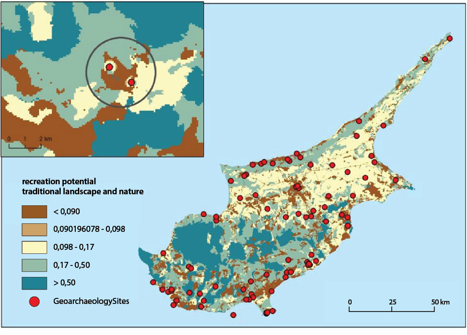
A map of recreation potential offered by the traditional cultural landscape and nature. This map is based on the recreation opportunity spectrum approach. The red dots are places of archaeological interest.
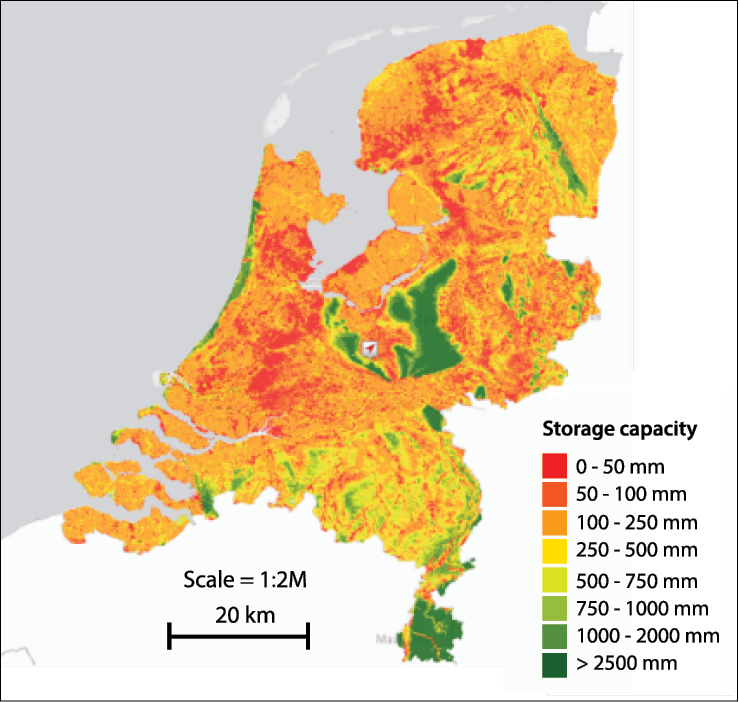
In the EU, countries have started initiatives to map their ecosystems and ecosystem services (ES) on their national territory. The principal objective is to create a national knowledge base on ecosystems which can be used for planning purposes such as the selection of areas for ecological restoration, the development of new infrastructure projects or land and water management. The European Commission is providing guidance to countries on how to map ecosystems and ES through the MAES initiative and collects information of countries on the biodiversity information system for Europe (http://biodiversity.europa.eu/maes).
Two examples for Cyprus and The Netherlands illustrate nation-wide mapping of ES in the EU. Cyprus is an island in the Mediterranean Sea. The map illustrates the recreational potential of the traditional landscape and nature. The map was made in a training workshop where country officials from the ministry worked together with scientists to map recreational services on the island. The Netherlands create maps of ES which are publicly available via their Atlas of Natural Capital (http://www.atlasnatuurlijkkapitaal.nl/en/home).
In the US, the Environment Protection Agency leads a multi-organisation effort to develop and host a suite of nationwide maps of ecosystem services (ES) indicators and indices in EnviroAtlas (https://epa.gov/enviroatlas). This open access tool allows users to view, analyse and download a wealth of geospatial data and other resources related to ecosystem goods and services. More than 160 national indicators of ecosystem service supply, demand and drivers of change provide a framework to form decisions and policies at multiple spatial scales, educate a range of audiences and supply data for research. A higher resolution component is also available, providing data for finer-scale analyses for selected communities across the US. The ecosystem goods and services data are organised into seven general ecosystem benefit categories: clean and plentiful water; natural hazard mitigation; food, fuel and materials; climate stabilisation; clean air; biodiversity conservation; and recreation, culture and aesthetics. EnviroAtlas incorporates many data sources with multi-resolution (i.e., 1 m and 30 m) land cover data providing fundamental information. The data are updated at 5 year increments, subsequent to US National Land Cover Dataset updates.
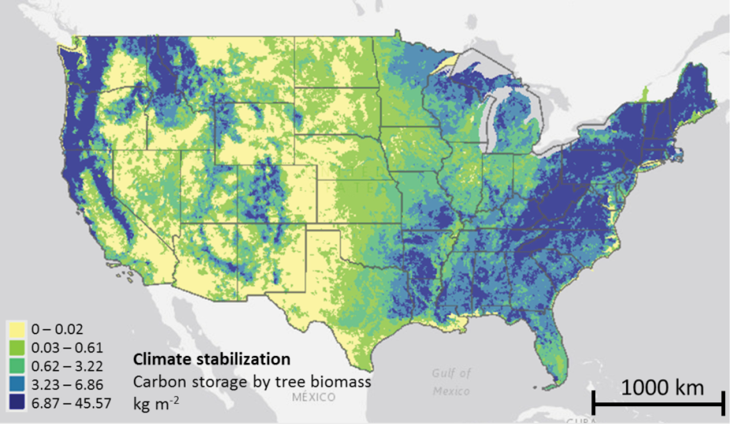
This map shows the kind of data layers that are available in EnviroAtlas. For one of the indicators in the climate stabilisation category, this map shows the amount of carbon stored in the above-ground tree biomass. Like most of the national maps in EnviroAtlas, the data are summarised by medium sized watershed drainage basins known as 12-digit hydrological unit codes (HUCS). There are approximately 85,000 of these HUCS in the conterminous US, with each being approximately 104 km?. Users of EnviroAtlas can also overlay demographic maps to gain the perspective of proximity and population dynamics of beneficiaries.
Conclusions
For the public, national maps can provide benefits that exceed their costs of production, assuming the maps are soundly executed, regularly updated and distributed to the public at a reasonable cost. When mapping ecosystems and ES at national levels, careful consideration should be given in the very early planning stages to the scale, accuracy and level of generalisation needed for the explicit and specific purpose the map is intended to serve. This is crucial when one considers that the degree to which a country acquires up-to-date and reliable knowledge of its ecosystems and ES will determine its ability to manage them. Mapping should not only provide information on the quality and quantity of ES but also on their distribution among the population within a country which is key to issues of equality and social justice. Usually, the loss of ES has the greatest impact on the poorest communities which, as a group, are the first to feel the effects when those ES begin to disappear. In this sense, the mapping of ecosystems at the national scale is essential to understanding the magnitude and spatial distribution of such services and for the development of policies to protect and restore them.
Finally, we stress that the most important investment a country can make when addressing these issues is on its human capital. The creation, maintenance, update and distribution of a national mapping initiative require trained, skilled, committed and motivated personnel, with technological considerations important but secondary. The human capital should have the highest priority.
Further reading
- Bailey RG (2009) Mapping Regional Ecosystems. Springer 2nd ED. DOI: 10.1007/978-0-387-89516-1.
- Burkhard B et al. (2009) Landscape's capacity to provide ecosystem services - a concept for land cover based assessments. Landscape on-line 151-22 DOI: 10.3097/lo.200915.
- EU biodiversity strategy to 2020 Mapping and Assessment of Ecosystems and their Services http://biodiversity.europa.eu/maes.
- Robinson AH et al. (1995) Elements of Cartography. New York: John Wiley and Sons, sixth edition.
- Schmidt S, Manceur A, Seppelt R (2016) Uncertainty of Monetary Valued Ecosystem Services - Value Transfer Functions for Global Mapping PLOS ONE March 3.
- Pickard BR, Daniel J, Mehaffey M, Jackson LA, Neale A (2015) EnviroAtlas: A new geospatial tool to foster ecosystem services science and resource management, Ecosystem Services 14: 45-55.
5.7.3. Global ecosystem service mapping approaches
Introduction
The global mapping of ecosystem services (ES) helps to diagnose management and conservation problems and develop solutions for them, as well as to analyse the impact of management decisions on biodiversity and ES. It enables the identification of synergies, trade-offs, hotspots of ES delivery and spatial mismatches between ES supply and demand or within world regions or sectors. Global initiatives (e.g. Convention of Biological Diversity and Millennium Ecosystem Assessment) make use of global ES maps to investigate the state and trends of global biodiversity and ES in order to formulate international policies. There is, consequently, an increasing demand for accurate maps of ES supply, demand and values. ES mapping is applied both for biophysical assessment of services and for valuation of these services. The history of global mapping of ES and their values globally dates back to the 1990s, concentrated on the monetary value of ecosystems. In the new millennium, global ES mapping studies were expanded to more biophysical descriptions. Although the number of publications targeting the mapping of ES has rapidly increased in the last years, global ES mapping remained limited to a few provisioning and regulating services (e.g. food provision, water availability and carbon sequestration). Obstacles for global ES mapping include the resolution of the available data, the uncertainty involved in upscaling local phenomena and the lack of knowledge of global ecological processes (see Chapter 6).
Various mapping approaches
A common approach for mapping ES is to quantify the relationships between ecosystem conditions (see Chapter 3.5) and ecosystem functions (i.e. the ecosystem's potential to provide a service, see Chapter 2.3) or services (i.e. the actual use of the function by humans; see Chapter 5.1). The mapping of ES often starts with maps of ecosystem types, land cover and land use. ES are then derived by applying models, quantifying each ES for each type of land use or land cover within each ecosystem. These models can either be simple correlative or expert-based models (see Chapter 4.6) or more complex process-based models (see Chapters 4.4 and 5.6.1). Developing these models is one of the main challenges for mapping global ES.
Global models are suitable tools for international science-policy assessments and decision-making support by assessing the impact of socio-economic drivers on the environment and ES. The Millennium Ecosystem Assessment used already-published individual models to assess the global ES trends and patterns. Others link sector-based global models to simulate the interaction between environmental processes and certain ES. Examples for global models are the Integrated Model to Assess the Global Environment (IMAGE IMAGE) developed by the PBL Netherlands Environmental Assessment Agency and the Global Unified Metamodel of the Biosphere (GUMBO pii/S0921800902000988) by the University of Maryland. The International Institute for Applied Systems Analysis (IIASA) has also developed several global models used in policy support, such as the Global Biosphere Management Model (GLOBIOM). Other efforts being applied to making decisions about ES in various case studies across the globe are the Natural Capital Project's InVEST, the ARtificial Intelligence for ES and The Earth Genome (see Chapter 4.4 for an overview of ES models).
Another common application of ES mapping is the creation of maps of monetary values (Chapter 4.3). Such approach is supposed to draw attention to the relative importance and the potential economic benefit that can be gained from ES, for example, when making choices on land management. The Benefit Transfer method is the simplest approach for ES value mapping. It estimates economic values by transferring existing estimates from studies already completed for (another) location. Values of various ES are aggregated to a constant value applied for an ecosystem or land cover type. The TEEB Valuation Database provides a Total Economic Value (TEV) for ES per global ecosystems or land covers.
Global ES modelled by IMAGE and GLOBIO-ES
IMAGE is one of the few integrated global models describing the impacts of socio-economic drivers on the environment. IMAGE has been used in combination with the global biodiversity model GLOBIO (http://www.globio.info/) to assess impacts of human activities on biodiversity captured by the Mean Species Abundance. Later, the model was extended with additional ES modules into the GLOBIO-ES model. IMAGE provides information about environmental drivers (e.g. climatic factors and land use allocation) that feed into GLOBIO and GLOBIO-ES. These models map biodiversity and ES at 0.5°x 0.5° spatial resolution and apply cause-effect relationships between the environmental variables, biodiversity and ES derived from literature. Currently, biodiversity and eleven ES can be assessed with the IMAGE-GLOBIO modeling framework. Although the models are strong in simulating the effects of changing socio-economic drivers and consequent biophysical and climate pressures on biodiversity and ES; the modelling of interactions between biodiversity and ES and between the various ES as well as the policy response to states of ES are missing links. The models have been applied for assessing biodiversity and ES at regional and global scale (https://www.cbd.int/gbo4/). Two concrete application examples of these models are presented in Boxes 1 and 2.
Challenges of global mapping
Mapping ES becomes more challenging with increasing extension of the mapped area, since less quantitative data and poorer knowledge of ecological and other processes are available and higher level of aggregation and simplification is necessary compared to regional and local scales.
Data availability and quality
Global ES modelling relies highly on land cover and land use data. Only few standard datasets exist and information on landscape structure, land use intensity and land management is poor or lacking. A widely used ecosystem or biome map is provided by the World Wildlife Fund (http://www.worldwildlife.org/biomes). A commonly used land cover and land use dataset is the Global Land Cover (GLC) 2000 map (http://forobs.jrc.ec.europa.eu/products/glc2000/ glc2000.php), which is also used in the Millennium Ecosystem Assessment and the IMAGE and GLOBIO-ES models. The TEEB Valuation Database uses the GlobCover dataset (http://due.esrin.esa.int/page_globcover.php).This dataset provides a higher-resolution alternative to the Global Land Cover, but it also has a lower thematic accuracy. There are also other databases available targeting certain ecosystem or land covers, such as the Global Lakes and Wetlands Database (http://www.worldwildlife.org/pages/glob al-lakes-and-wetlands-database), the World Database of Protected Areas (http://www.protectedplanet.net/), the livestock density database of the Food and Agriculture Organisation of the United Nations (FAO) (http://www.fao.org/ag/AGAInfo/resources/en/ glw/GLW_dens.html) and forest cover datasets (e.g. http://www.globalforestwatch.org). Due to the limited data availability, the same datasets are often used for multiple purposes, which can lead to autocorrelations. Global data include increased uncertainty as they are often estimated or modelled (e.g. FAO livestock data). Uncertainty can be addressed with sensitivity analyses (see Chapter 6.3), but is not often done in practice. Last but not least, it remains difficult to validate global datasets due to differences in temporal and spatial consistencies and classification systems, amongst others.
Ecological processes and ES: knowledge and scale at which they operate
The knowledge of ecological and other processes becomes more limited with increasing extension of the mapped area. ES that operate based on well-known global processes, such as the hydrological or carbon cycle, are easier to map globally. Furthermore, global maps are more easily generated if an ES can be aggregated across time or space. This is the case for several provisioning services, such as crop, timber or livestock production. For these ES, monetary value maps can also be prepared, as their products are traded on markets.
ES that operate locally are, however, more difficult to map globally. ES such as pest control and air quality regulation are rarely considered globally because of the lack of generalised knowledge and the local scale at which they operate. Pollination and pest control are dependent on small-scale landscape elements making it difficult to map them accurately globally. Furthermore, cultural services such as aesthetic value, recreation and tourism have a subjective and local character which makes them difficult to generalise. As these ES do not have a direct market value either, it is more difficult to prepare a monetary value map for them.
Little generalised information is available about the degradation of ecosystem functions over time and the inter-linkages between biodiversity and ES and between the various ES. Degradation is, therefore, not fully addressed and biodiversity and ES are mainly modelled and valued separately at global scale. An approach to address these inter-linkages between ES is to create hotspot maps (i.e. highlighting areas where multiple services are provided).
Conclusions
Various approaches exist for the global mapping of ES, the most common ones being the biophysical and monetary value maps. Despite the limited data and knowledge available at global scale, global ES maps remain an important input for international science-policy assessments and for awareness-raising. Global models have the capacity to simulate ES trends across space and time and to identify ES synergies, trade-offs and values. This makes them essential tools for decision-making about resource management and nature conservation across the globe.
Figure
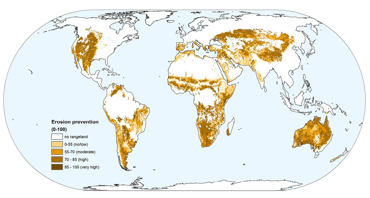
With the help of scenarios, the trends of ES delivery can be projected over time. In this example, the global crop production is simulated with the IMAGE and GLOBIO-ES models for two future scenarios. The production of cereals, rice, maize, pulses, root and tubers is taken as an indicator of crop production. The demand for crops is driven by changing lifestyle and population, whereas technology, environmental factors and management determine the production efficiency hence the crop yield. The two scenarios are adjusted SSP scenarios (i.e. new IPCC scenarios) used in the OpenNESS EU project. The 'Wealth-Being' (WB) scenario stands for economic growth, while the 'Eco-Centre' (EC) scenario promotes sustainable management around the globe. Figure
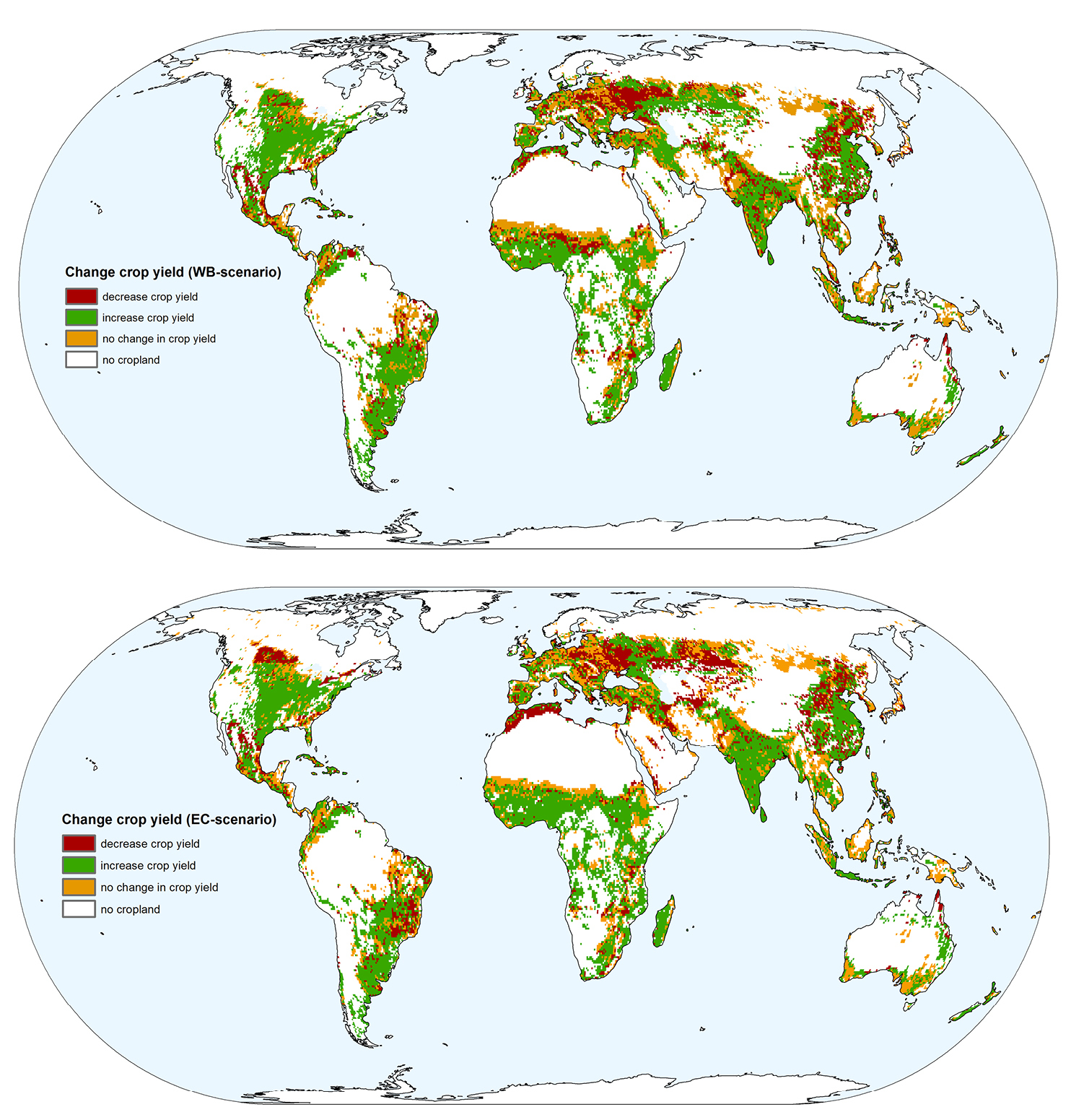
Further reading
- Alkemade R, van Oorschot M, Miles L, Nellemann C, Bakkenes M, ten Brinket B (2009) GLOBIO3: A Framework to Investigate Options for Reducing Global Terrestrial Biodiversity Loss. Ecosystems 12(3): 374-390.
- De Groot R, Brander L, van der Ploeg S, Costanza R, Bernard F, Braat L, Christie M, Crossman ND, Ghermandi A, Hein L, Hussain S, Kumar P, McVittie A, Portela R, Rodriguez LC, ten Brink P, van Beukering P (2012) Global estimates of the value of ecosystems and their services in monetary units. Ecosystem Services 1: 50-61.
- Dickson B, Blaney R Miles L, Regan E, van Soesbergen A, Vaananen E, Blyth S, Harfoot M Martin CS, McOwen C, Newbold T, van Bochove J (2014) Towards a global map of natural capital: key ecosystem assets. UNEP, Nairobi, Kenya.
- Kok M, Alkemade R (Eds.) (2014) How Sectors can contribute to sustainable use and conservation of biodiversity, CBD Technical Series.
- Naidoo R, Balmford A, Costanza R, Fisher B, Green RE, Lehner B, Ricketts TH (2008) Global mapping of ecosystem services and conservation priorities. Proceedings of the National Academy of Sciences 105(28): 9495-9500.
- Petz K, Alkemade R, Bakkenes M, Schulp CJ, van der Velde M, Leemans R (2014) Mapping and modelling trade-offs and synergies between grazing intensity and ecosystem services in rangelands using global-scale datasets and models. Global Environmental Change 29: 223-234.
- Turner WR, Brandon K, Brooks TM, Costanza R, Da Fonseca GA, Portela R (2007) Global conservation of biodiversity and ecosystem services. BioScience 57(10): 868-873.
- Schagner JP, Brander L, Maes J, Hartje V (2013) Mapping ecosystem services' values: Current practice and future prospects. Ecosystem Services 4: 33-46.
- Schulp CJE, Alkemade R (2011) Consequences of uncertainty in global-scale land cover maps for mapping ecosystem functions: an analysis of pollination efficiency. Remote Sensing 3: 2057-2075.
- Schulp CJ, Alkemade R, Klein Goldewijk K, Petz K (2012) Mapping ecosystem functions and services in Eastern Europe using global-scale data sets. International Journal of Biodiversity Science, Ecosystem Services & Management 8(1-2): 156-168.
- Stehfest E, van Vuuren D, Bouwman L, Kram T (2014) Integrated assessment of global environmental change with IMAGE 3.0: Model description and policy applications. Netherlands Environmental Assessment Agency (PBL).
- Verburg P, van Asselen S, van der Zanden E, Stehfest E (2012) The representation of landscapes in global scale assessments of environmental change. Landscape Ecology 28: 1067-1080.
- Verburg PH, Neumann K, Nol L (2011) Challenges in using land use and land cover data for global change studies. Global Change Biology 1: 974-989.
5.7.4. Mapping marine and coastal ecosystem services
Introduction
The marine environment, from the coasts to the open ocean, is closely tied to human well-being; from small-scale artisanal fisheries providing local communities with food, to large-scale regulating benefits like protecting coasts from erosion and regulating global climate. Intense human intervention in these areas, for example, through maritime transport, fishing and aquaculture, oil extraction, tourism and coastal land use, alter these ecosystems, hence impacting human well-being. Several treaties and policy instruments have been enacted from the local to global level to regulate human influence on the marine realm and to sustain these ecosystems (for example, the UN Convention of the Law of the Sea, the UN High Seas Treaty). In addition, the EU Marine Strategy Framework Directive and that on Maritime Spatial Planning require an ecosystem-based approach to the management of human activities.
Mapping of ES can help decision-makers define critical areas for intervention and aids regulation of activities. Although mapping methodologies are rapidly advancing for the terrestrial and inland water ecosystems, marine and coastal ecosystem service (MCES) mapping is still limited.
This chapter gives an overview of MCES mapping principles. We present below the major ES provided by marine and coastal habitats, the particularities and differences of MCES mapping compared to the terrestrial realm and its major requirements and limitations.
ES provided by marine and coastal habitat types
Each marine or coastal habitat type can generate different ecological functions which can then generate ES for the benefit of human beings. In Table
Major marine and coastal habitat types and their links with ES as documented in the literature. The (u) symbol represents the relationships between habitat types and ES that have been assessed and documented in the literature. The (?) is there to represent the lack of sufficient knowledge to assess and hence quantify and map this relationship.
* These habitats and ES are still very poorly analysed.
| Provisioning | Regulating and maintenance | Cultural | |||||||||||
|
Food provision
|
Water storage / provision
|
Biotic materials/Biofuels
|
Water purification
|
Air quality regulation*
|
Coastal protection
|
Climate regulation
|
Ocean nourishment
|
Life cycle maintenance
|
Biological regulation*
|
Recreation Tourism
|
Symbolic/Aesthetic values
|
Cognitive effects
|
|
| Beach and dunes | ? | ? | ? | ? | ? | ? | ? | ? | ? | ? | ? | ? | ? |
| Coastal wetland | ? | ? | ? | ? | ? | ? | ? | ? | ? | ? | ? | ? | ? |
| Estuary | ? | ? | ? | ? | ? | ? | ? | ? | ? | ? | ? | ||
| Mangrove | ? | ? | ? | ? | ? | ? | ? | ? | ? | ? | ? | ? | ? |
| Coral Reef | ? | ? | ? | ? | ? | ? | ? | ? | ? | ? | ? | ? | ? |
| Maerl bed* | ? | ? | ? | ? | ? | ? | ? | ? | ? | ? | ? | ? | ? |
| Oyster reef | ? | ? | ? | ? | ? | ? | ? | ? | ? | ? | ? | ? | ? |
| Macroalgal bed | ? | ? | ? | ? | ? | ? | ? | ? | ? | ? | ? | ? | ? |
| Seagrass meadow | ? | ? | ? | ? | ? | ? | ? | ? | ? | ? | ? | ? | ? |
| Unconsolidated sediments | ? | ? | ? | ? | ? | ? | ? | ? | ? | ? | ? | ? | ? |
| Open ocean pelagic | ? | ? | ? | ? | ? | ? | ? | ? | ? | ? | ? | ? | ? |
Mapping marine and coastal ecosystem services
To map ES provided by marine and coastal ecosystems similarly to the terrestrial ecosystems, one has to understand the process of ES provision, from the ecosystem components, functions and processes to the actual ES. For each component of the ES provision chain, data need to be acquired and quantification methods applied throughout. This information can be used to spatially represent the ES distribution. In Figure
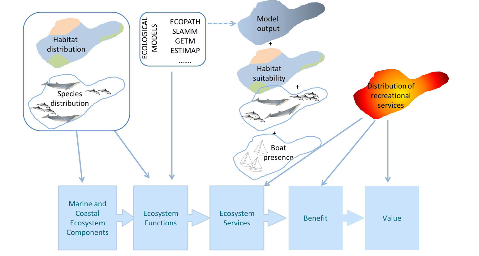
The figure depicts the way data and ecological models contribute to the different components of a basic ecosystem service generation framework (ES cascade at the bottom of the figure) in order to generate ES maps. In an example of whale watching tourism as an ES provided by whales, species and habitat distribution models are used to describe the basic ES components. Then models are used to describe the ecosystem functions. The outputs of all these models are then combined along with socio-economic parameters (in the example we refer to the number of whale watchers, but it could also be revenues from whale watching) in order to generate a final map of the benefit or value from whale-watching tourism. The arrows show the flow of information within the elements of the ES cascade.
In the oceans and coastal seas, many ecosystem functions occur within the water column which adds a third spatial dimension to the system. These functions change with depth, water temperature, solar irradiance, salinity and other factors and are extremely variable in space and time. This makes it difficult to capture this information in two-dimensional maps.
MCES maps are delivered by:
Analysis of primary data, for example, high resolution remote sensing of the coastal and pelagic zone, field sampling and socio-economic surveys. It can be very accurate, but it is also time and resource consuming.
Habitat maps can be used to translate seabed habitat maps into capacity to deliver ES based on scoring factors. This method can be feasible and quick if the seabed habitat maps of the study area are already available. However, the scoring system can be subjective and the results reflect only the services provided by benthic habitats.
Modelling
Models such as those below can be used:
Ecosystem models optimally integrated with socio-economic data, or bio-economic models. They can be relatively accurate with quantifiable uncertainty and capture three-dimensional (3D) processes across spatial scales. Still they require a lot of data, time and expertise. Model outputs may not be usable as such; composites or proxies often need to be generated for MCES mapping.
Already available MCES mapping tools (see the following section).
Most MCES maps depict the ES capacity and very few address the actual flow of, or the demand (Chapter 5.1) for MCES. The analysis of all these ES aspects is essential, especially for MCES whose use is often distant from the source of ES provision (e.g. the nutritional value of globally consumed tuna or climate regulation by mangroves in South-East Asia).
Required data for MCES mapping
The possibility of creating MCES maps is often limited due to scarcity of spatial data. For proper ES mapping, data should ideally be available for:
Habitats' spatial distribution (or their model-derived proxies);
ecological state of the habitats;
water quality affecting ES provision (e.g. eutrophication or amount of harmful substances);
species distribution of dominant, habitat forming and keystone species that either provide or support ES;
biomass of fish and other seafood;
human activities affecting the production of ES or those which could be used as indicators for ES use (e.g. fishing activity, tourism etc.).
Collecting such data is laborious and expensive, mostly because of the methodological challenges. Some examples are given in the following text.
Data on benthic habitats need to be collected with echo-sounding methods and tedious geological analysis of the sonar data. Species data need to be collected with a suite of methods that vary in spatial coverage and taxonomic accuracy. Data on sea bottom substrate and larger species can be collected with underwater cameras, while information on smaller species can be derived with underwater surveys (e.g. through scuba diving) and benthic sampling. Species identification often requires microscopic analysis.
Some proxies for ES can be created for more cost-effective methods. The new satellite instruments provide high resolution data (e.g. WorldView3 images have a resolution of 30 cm) that can be used to create proxies for some ES, like habitats essential for fish production. Semi-automatic in situ mapping devices, such as robot gliders, have been developed for collecting sea bottom data instead of cruises on research vessels. Such methods can complement, but never entirely replace, the traditional methods.
Spatial data on certain human activities can easily be derived from public databases, but in most cases data are scarce. Proxies need to be calculated although these create uncertainties in the mapping.
MCES mapping tools
Different online tools, models and methodological frameworks allow practitioners to assess and map different components of the MCES generation chain (Figure
Several initiatives focus on publishing spatially explicit information regarding or potentially supporting MCES mapping. The SeaAroundUs (http://www.seaaroundus.org/data/#/spatial-catch) project has released a map server showing time series of the spatial distribution of fisheries around the globe. The EU has recently released a new tool for mapping fishing activities (MFA) for the European seas which is based on AIS (Automatic Identification System) data acquired by fishing vessels. AquaMaps also provide maps of marine species distribution globally. The Baltic Sea data and map service, by the Helsinki Commission, provides spatial data on biodiversity and human activities on sea. The Ocean Health Index Project provides a global map of ES provided by the sea and how sustainably the countries are using them.
Challenges of MCES mapping
There is a high level knowledge pool on the functioning of the marine ecosystems and high expertise on ES mapping methods. Yet these two only recently started converging in an interdisciplinary manner. Hence the number of MCES assessments that actually provide maps is still very limited. Challenges to MCES mapping include:
The dynamic three-dimensional (3D) nature of the marine environment, especially in the pelagic zone, makes it difficult to produce two-dimensional maps. Averaging over time and space is necessary and hence the level of spatial accuracy is low.
Information on the distribution of habitat is scarce or entirely lacking making it difficult to map MCES based on these habitats.
As the ecological functions and processes behind many ES, such as biological regulation, are not known or not easily quantified, their mapping is difficult.
Cultural ES, such as recreation, aesthetic information or inspiration, are based on human experiences which may be very variable. Linkage of such experiences to a specific habitat is difficult.
Data on ES demand or use is sensitive thus hard to obtain for some ES with high commercial value (e.g. food provision from fisheries).
Uncertainty in data and maps is too high to be useful in a policy context, therefore having often a negative feedback effect on momentum to create these maps.
Future recommendations
Given the limited number of MCES maps, there is a need to:
Adapt the current ES methodologies and frameworks that have been developed based on terrestrial ecosystems to the specificities of the marine environment.
Improve the quality and spatial resolution of data and improve data availability; advance initiatives such as the European Marine Knowledge 2020; and feed data into harmonised databases like the EMODNET (http://www.emodnet-biology.eu/) data portal.
Adopt a holistic view of the ES provision chain focusing on the intermediate steps (from the ES to the benefit). In particular, the valuation of regulating services and the ecological processes supporting provisioning and cultural services should be reinforced.
Communicate the uncertainties in MCES maps. Explain how much of the spatial detail shown on maps is reliable. Recommend for which purpose the maps can - and cannot - be used.
Further reading
- Bohnke-Henrichs A, Baulcomb C, Koss R, Hussain SS, de Groot RS (2013) Typology and indicators of ecosystem services for marine spatial planning and management. Journal of Environmental Management 130: 135-145.
- Boonstra WJ, Ottosen KM, Ferreira ASA, Richter A, Rogers LA, Pedersen MW, Kokkalis A, Bardarson H, Bonanomi S, Butler W, Diekert FK, Fouzai N, Holma M, Holt RE, Kvile KO, Malanski E, Macdonald JI, Nieminen E, Romagnoni G, Snickars M, Weigel B, Woods P, Yletyinen J, Whittington JD (2015) What are the major global threats and impacts in marine environments? Investigating the contours of a shared perception among marine scientists from the bottom-up. Marine Policy 60: 197-201.
- Liquete C, Piroddi C, Drakou EG, Gurney L, Katsanevakis S, Charef A, Egoh B (2013a) Current Status and Future Prospects for the Assessment of Marine and Coastal Ecosystem Services: A Systematic Review. PLoS ONE 8: e67737.
- Liquete C., Zulian G., Delgado I., Stips A., Maes J. (2013) Assessment of coastal protection as an ecosystem service in Europe. Ecological Indicators 30: 205-217.
- Townsend M, Thrush SF, Lohrer AM, Hewitt JE, Lundquist CJ, Carbines M, Felsing M (2014) Overcoming the challenges of data scarcity in mapping marine ecosystem service potential. Ecosystem Services 8: 44-55.
5.7.5. Spatial, temporal and thematic interactions
The role of spatial and temporal scales in ES mapping; scale dependencies of different (groups of) ES
Ecosystem services (ES) are scale-dependent. While a single tree can have a positive impact on the micro-climate (local scale), it does not necessarily impact the climate regulation at global scale. Interactions of spatial and temporal scales make the mapping of ES more complex. Therefore, without taking into account the age of a tree and its relations with other trees or other land uses (landscape scale/regional scale), no precise statement on its contribution to climate regulation can be derived across scales. Additionally, scale dependence is related to different perspectives, including the ES provider (supply) and the ES beneficiary (demand), as well as ES assessment (expert) and ES management (stakeholder). In this chapter, we assess and clarify the various aspects of scale interactions and perspectives in the context of ES mapping.
The difficulty of scale interactions lies in many aspects. The mapping exercise as such can be conducted in a straightforward manner at many scales; the greater challenge is the data availability. Regarding scales, the assessment of ES at the local scale is sometimes easier, because systems are smaller and thus better investigated, understood and supported by data. At the regional scale, spatial interactions between various ecosystems make the ES investigation more difficult, as boundary phenomena between ecosystems or land use types have been less investigated. Knowledge and data about the influence of composition and configuration of land use types remains limited (see Chapter 3.6). For assessing ES at continental or global scales (see Chapter 5.7.3), ES data from local, regional and national assessments (see Chapters 5.7.1 and 5.7.2) need to be up-scaled. Therefore, mapping and assessment of ES at global scale might involve high uncertainty. Additionally, indicators which are used to assess ES, are in many cases scale-sensitive.
Furthermore, the beneficiaries as well as the perception of ES benefits change across scales: supply and demand are largely scale-dependent. At local scale, individuals might be directly dependent from provisioning services such as food or water ("private ES") so that their activities (land management, purchase) are directed towards harmonising the spatio-temporal variation between supply and demand. Global services, such as global climate regulation, are relevant for humanity ("public services"). Their spatial and temporal dynamics, also called "spatio-temporal lag", are huge (see Chapter 5.2). Consequently, their perception and appreciation have the character of a shared value which complicates their assessment and the application of financial instruments such as Payments for Ecosystem Services (PES) to boost them (Table
Generalised scheme of the antagonism of ES awareness across spatial scales. *and further local actors and stakeholders
| Scale | Measurement | Perception of benefits | Beneficiary | Payment for ES |
| Local | Easy | Good | Land owner* | Feasible |
| Regional | ||||
| National | ¦ | ¦ | ¦ | ¦ |
| Continental | ||||
| Global | Difficult | Poor | Human kind | Difficult |
In land management and land use planning, the ES concept contributes to the assessment of sustainability from a highly integrative perspective that covers regulating, provisioning and cultural ES and allows the assessment of the value of biodiversity as a supportive backbone to enable ES supply (see Chapter 2.2). A multitude of indicators (e.g. in the context of CICES 4.3 (http://cices.eu/), Chapter 2.4) has been introduced for the different service groups. However, many of them address a specific scale so that the subsequent assessments require intense data collection, analysis and aggregation. Taking regulating services as an example, "mediation of smell/noise/visual impacts" relates to local or regional scale, while "dilution by atmosphere, freshwater and marine ecosystems" refers to regional, national or even global scale.
In this chapter, we explore how to integrate data from different scales in a comprehensive manner. Using the results from the project RegioPower (www.eli-web.com/RegioPower/) as an example, in Boxes
In RegioPower, we focussed on exploring regional biomass provisioning capacities and focus here on the service "timber production". Measured or modelled data, as well as stakeholder experience or expert opinion can serve as the basis for the assessment of this service. We made use of forest inventory data and regional statistics (harvesting, trade) and included empirical data when no specific information could be obtained. Through normalisation, this quantitative information basis can be adjusted for trade-off analyses with other services, such as "Aesthetics" or "Carbon sequestration". Subsequently, with the help of the software GISCAME (www.giscame.com), the effective capacity of providing services bundles and their balance can be assessed in a spatially explicit manner or as summary information at regional scale. This approach of local data collection and subsequent normalisation for up-scaling to larger scales (Figure
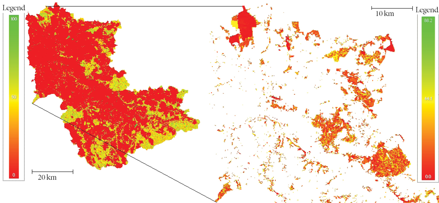
Scale interactions
To move from local data to regional decision support, various data need to be collected, harmonised and integrated. Data might encompass measured data from field studies, empirical data from surveys, modelled data, or expert judgements if quantitative data is not available. Hence, the first challenge is the identification of adequate indicators. Regarding spatial reference, a cross-scale approach might be necessary, for example, the collection of local data, in order to regionalise them for an ES assessment at the regional or national scale (Box
Once the status quo of ES is assessed and mapped, the next challenge is the consideration of the temporal scale (Box
In addition to space and time, thematic interactions need to be taken into account to avoid unexpected trade-offs (Box
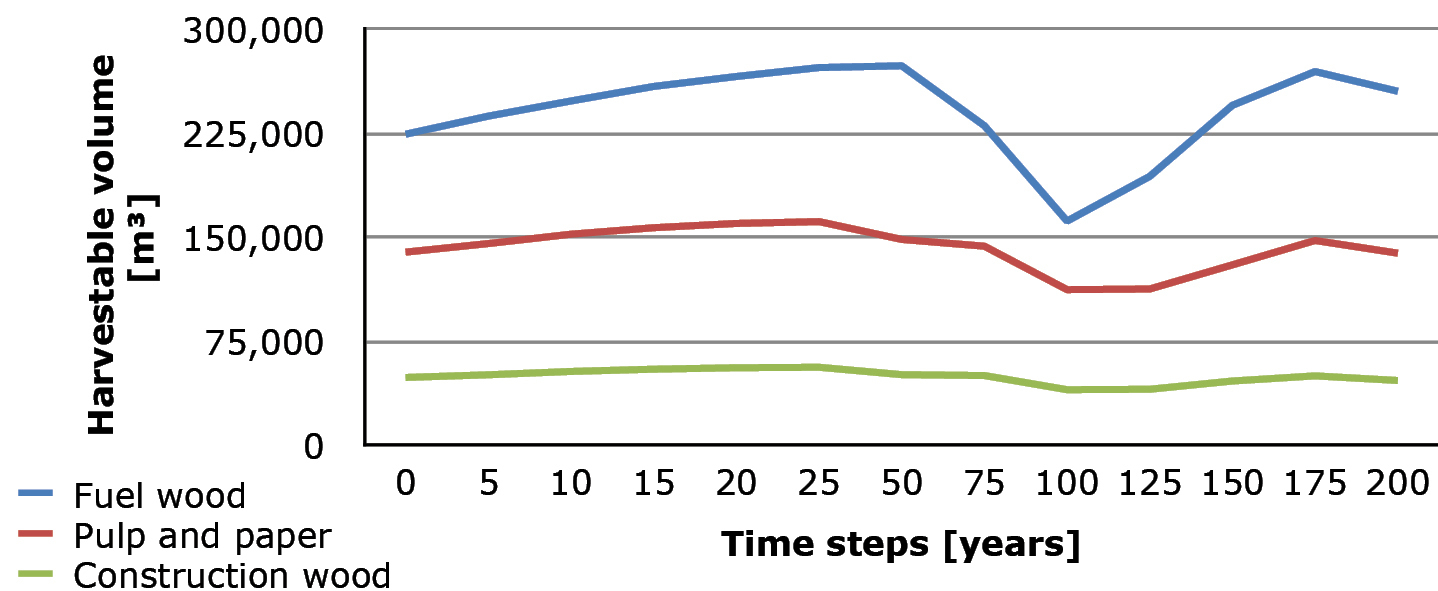
Temporal variation of the provisioning service "timber provision" considering three timber assortments.
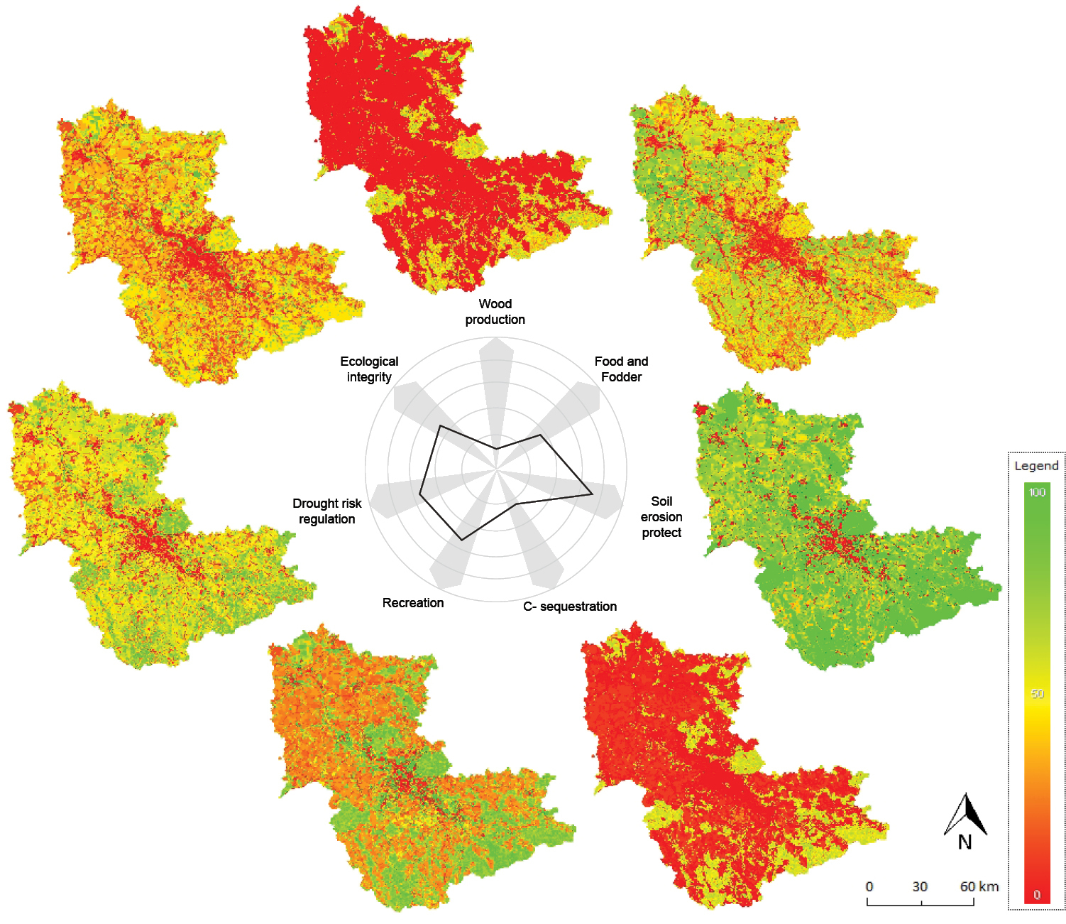
Conclusions
For a holistic and reliable assessment of ES, it is crucial to consider the sensitivity of underlying indicators to spatial and temporal scales. Only scale-appropriate land use planning including proper land management practices can ensure the sustainable provision of ES. Spatially explicit tools that support integrating models from different land use sectors and aggregating qualitative and quantitative information are required to support informed decision-making processes.
Future challenges in providing reliable information on ES supply capacities include a stronger consideration of boundary phenomena (proximity effects) whose impacts on the availability of ES are often ignored due to the lack of respective monitoring data. In addition, the impact of the landscape configuration on ES supply capacities (see Chapter 3.6) as a key research topic of landscape ecology should be more actively reflected in ES assessments. Regulating and cultural ES, as well as provisioning services, are highly dependent on compactness or fragmentation that can accelerate or diminish, for instance, the productivity of forest or agricultural land.
There is still a need to develop appropriate governance models to ensure the provision of ES that are not directly consumed and thus are often underestimated in their relevance, such as many regulating ES (see Chapter 5.5.1). Particular services that represent shared, public values, such as global climate regulation (which cannot easily be directly connected to beneficiaries) require societal agreement on how to deal with discrimination of land owners who would need to renounce economic benefits from land use for the sake of the global population. Spatially explicit modelling and integrated assessments of ES which could support identifying areas and subsequently their owners are of particularly high value for providing such critical services. Global agreements and strategies on how to compensate potential restrictions, for example, in tropical or boreal forest areas, should consequently be developed.
Further reading
- Frank S, Furst C, Pietzsch F (2015) Cross-sectoral resource management: how forest management alternatives affect the provision of lignocellulosic resources and other ecosystem services. Forests 6: 533-560.
- Fremier AK, DeClerck FAJ, Bosque-Perez NA, Carmona NE, Hill R, Joyal T, Keesecker L, Klos PZ, Martinez-Salinas A, Niemeyer R, Sanfiorenzo A, Welsh K, Wulfhorst JD (2013) Understanding Spatio-temporal Lags in Ecosystem Services to Improve Incentives. BioScience 63: 472-482.
- Furst C, Frank S, Rozas-Vasquez D, Jimenez M, Pietzsch K, Pietzsch F (2016) How to assess the impact of agricultural and forest management on biodiversity and ecosystem services. In: Geneletti D (Ed.) Handbook on biodiversity and ecosystem services in impact assessment. Edward Elgar Publishing, 195-221.
- Gret-Regamey A, Weibel B, Bagstad KJ, Ferrari M, Geneletti D, Klug H et al. (2014) On the Effects of Scale for Ecosystem Services Mapping. PLoS ONE 9(12): e112601. doi: 10.1371/journal.pone.0112601.
- Gret-Regamey A, Weibel B, Kienast F, Rabe S-E, Zulian G (2015) A tiered approach for mapping ecosystem services. Ecosystem Services 13: 16-27.
- Hayek UW, Efthymiou D, Farooq B, von Wirth T, Teich M, Neuenschwander N, Gret-Regamey A (2015) Quality of urban patterns: Spatially explicit evidence for multiple scales. Landscape and Urban Planning 142: 47-62.
- Malinga R, Gordon LJ, Jewitt G, Lindborg R (2015) Mapping ecosystem services across scales and continents - A review. Ecosystem Services 13: 57-63.
- Norton L, Greene S, Scholefield P, Dunbar M (2016) The importance of scale in the development of ecosystem service indicators. Ecological Indicators 61(Part 1): 130-140.
Chapter 6. Uncertainties of ecosystem services mapping
6.1. Data and quantification issues
Introduction
Chapters 4 and 5 describe many different methods and approaches for mapping ecosystem services (ES) across time and space. However, as with any mapping exercise, the usefulness of the map is only as good as the input data ("garbage in, garbage out"). It is important to be aware of the common data and quantification challenges when making ecosystem service maps to prevent production of poor quality maps.
The aim of this chapter is to discuss some of the common challenges quantifying ES for use in maps. The chapter principally focuses on challenges when data is scarce and/or system understanding is poor. Challenges relating to scale are also considered, such as the Modifiable Area Unit Problem (MAUP; see also Chapter 3.2) and the ecological fallacy, the importance of metadata (data about data) and the need to avoid double-counting of ecosystem service values in maps. This chapter will offer solutions to these problems, including a list of online spatial data resources to fill data gaps.
Limited data
It is a general principle that wealthier countries and regions with advanced economies will have higher resolution and more accurate spatial data that can be used to map ES. There will often be readily accessible high resolution climate, topography, soil, biodiversity, land use and land cover data. Data acquisition will be at relatively low cost and data may even be available free of charge when governments commit to open data policies.
In locations where there is a lack of ecosystem service data, it will be necessary to fill data gaps with alternative approaches such as remote sensing, participatory mapping, land use proxies and/or use of lower resolution global-scale datasets. Creative ways to fill data gaps are needed when ecosystem service mapping projects have limited resources to collect new data and build new models.
Filling data gaps
Participatory mapping
Participatory mapping, or participatory GIS, is an increasingly popular technique for collecting data on ES using local expert knowledge (see Chapter 5.6.2). A participatory mapping exercise involves bringing together local expertise in a workshop setting and capturing on maps (paper or digital) experts' understanding of the spatial distribution of ES of interest. Figure
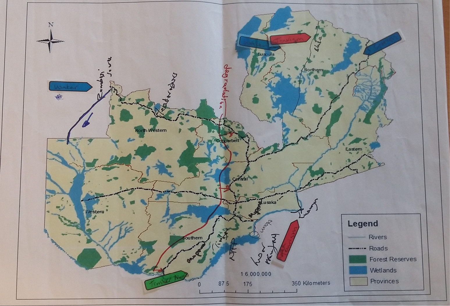
Example of paper map used in a participatory mapping exercise to map ecosystem service and land degradation management priorities in Zambia (Source: Willemen et al. 2015).
Often the cultural ES have the least data and understanding and participatory approaches are best suited to capture that category of services. A recent review of 30 participatory GIS ecosystem service mapping case studies found that multiple methods were implemented and cultural and provisioning services were most commonly mapped.
Participatory approaches have the extra benefit of adding acceptance and credibility to ecosystem service mapping because they include and capture local knowledge.
Remote sensing
Remotely sensed satellite data can be used to fill data gaps but the data are limited by what can be captured from above the land surface. Remotely-sensed data are often used to derive spatial estimates of many ES such as food production (mapping of crops), surface and ground water (mapping of water bodies and watercourses), vegetation cover and attributes (vigour, biomass), soil condition and erosion, flood control (mapping of floodplain topography) and coastal protection (mapping of mangrove and dune systems). Land cover and land use are common datasets captured by remote sensing and these data can act as proxies for mapping the supply of ES. The land cover/land use approach to mapping ES is a common and very useful technique in the absence of detailed spatial models, data and system understanding.
Global scale data
Many global scale datasets are available for mapping ES, although their usefulness will be determined by the scale of mapping required (Chapter 5.7). Global scale data is typically of coarse resolution (from 1 km resolution and above), so mapping at local scales will often prohibit the use of global scale datasets. Global data will be more useful for mapping at national/regional/continental scales. A list of global datasets useful for mapping ES is provided in Table
Selection of global datasets for mapping ES (note: some datasets require post-processing to estimate ES).
Scale issues
The Modifiable Areal Unit Problem (MAUP)
The aggregation of spatial point data into arbitrary spatial units such as postcode areas, suburbs or ecosystem types introduces a bias known as the Modifiable Areal Unit Problem (MAUP). The boundaries of the aggregated unit are arbitrary, modifiable and therefore drawn at the discretion of the person undertaking the aggregation. The result is that the summary values for each areal unit are influenced by the choice of unit boundary leading to the display of data in maps which can be misleading. Aggregation of the same data to different boundaries could lead to very different summary data and maps. Figure
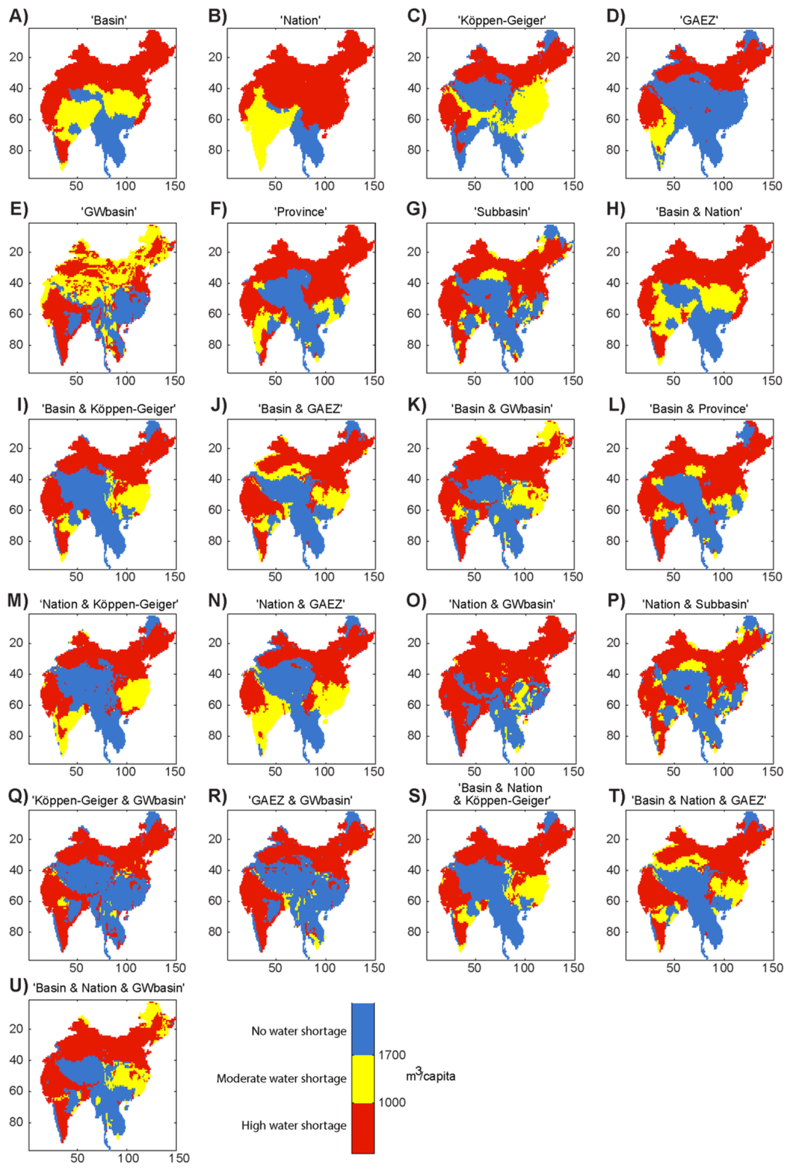
Example of the MAUP across 21 different boundaries in Asia. Extent of water shortages (m3/cap/year) can be very different depending on choice of boundary (Source: Salmivaara et al. 2015).
Ecosystem service maps are vulnerable to MAUP where point-based data (or high-resolution raster data) is aggregated to large spatial units. Obvious examples are food production, freshwater abstractions, point-sourced pollution and pollution treatment, tourism and recreation activity, and species habitat; but all ES could be affected by MAUP if their maps summarise high-resolution information to coarse, arbitrary boundaries. Although sophisticated models and techniques are available to accurately interpolate and summarise point-based and high resolution spatial data (such as geographically weighted regression), the simplest approach is to recognise the MAUP in the first place and then to ensure the areal units into which data is summarised are as internally homogenous as possible.
Ecological fallacy
Related to the MAUP is another data aggregation and scaling issue known as the ecological fallacy. Here a logical fallacy occurs when inferences about data at the individual (or local) scale are made from population-level (or coarse-scale) data.
The ecological fallacy occurs because it is easy to make the erroneous assumption that relationships between variables at a coarse level of aggregation also hold for lower levels of aggregation. For example, at a coarse level, there may be a strong relationship between increasing crime rates and lower income levels; yet it would be wrong to conclude that lower income individuals are more likely to commit crime because participation in crime is a function of many other variables, not just income level.
In ecosystem service mapping, an ecological fallacy could arise when mapping the value of coastal protection by mangroves. It would be a fallacy to assume all mangroves in a coastal area offer storm protection based on the coarse level positive relationship between mangrove area and level of storm protection. The level and, therefore, the value of storm protection at discreet locations within mangrove systems, is a function of other variables such as topography and distance to shoreline.
Documenting mapped data
The rapid growth in ES research and implementation risks being undermined by poor data management and mapping practices. There is a recognised inconsistency in ecosystem service modelling and mapping methods which limits the use of ecosystem service information in national accounts and policy decision-making related to the environment. A basic set of metadata should be recorded during every ecosystem service quantification and mapping study. For example, information about the mapping study, such as purpose, location, duration, administrative unit mapped, citations and project investigators should be recorded and published with the maps. For each ecosystem service modelled/mapped, attributes such as ecosystem service indicator, data source, quantification unit and method, scale, extent, resolution, time period and beneficiary definition should be recorded on a blueprint. Completing metadata and blueprints for ES quantification/mapping will provide users of the data and maps with a confidence in the pedigree and usefulness of the information.
Producing metadata and blueprints as part of a mapping exercise provides a level of standardisation of the data for easy inclusion in catalogues such as the ESP Visualisation Tool (ESP-VT). The ESP-VT is an online web portal and catalogue for uploading, downloading and querying spatial information on ES (Chapter 7.9). Another important cataloguing tool is the Intergovernmental Platform on Biodiversity and Ecosystem Services (IPBES) Catalogue of Assessments. The IPBES Catalogue aims to build a global database of studies of ecosystem service quantification and valuation.
Double-counting
Double-counting is an economics term that refers to the erroneous practice of counting the value of goods or services more than once. Double-counting of ecosystem service values arises, for example, when supporting or intermediate ES such as soil formation, nutrient cycling and photosynthesis are valued and mapped in conjunction with the valuation and mapping of final ES. The problem of double-counting also occurs when there is overlap between ES because of vague service definitions and categorisations and/or limited understanding of ecosystem functions and processes. Recent classification systems such as CICES and the US EPA's FEGS-CS have taken considerable care to ensure final ES are clearly categorised to minimise the likelihood of double-counting in valuation and mapping.
Further reading and resources
- Brown G, Fagerholm N (2015) Empirical PPGIS/PGIS mapping of Ecosystem Services: A review and evaluation. Ecosystem Services 13: 119-133.
- Crossman ND, Burkhard B, Nedkov S, Wil- lemen L, Petz K, Palomo I, Drakou EG, Martin-Lopez B, McPhearson T, Boyanova K, Alkemade R, Egoh B, Dunbar M, Maes J (2013) A blueprint for mapping and modelling Ecosystem Services. Ecosystem Services 4: 4-14.
- Drakou EG, Crossman ND, Willemen L, Burkhard B, Palomo I, Maes J, Peedell S (2015) A visualisation and data-sharing tool for ecosystem service maps: Lessons learned, challenges and the way forward. Ecosystem Services 13: 134-140.
- Fu B-J, Su C-H, Wei Y-P, Willett IR, Lu Y-H, Liu G-H (2011) Double counting in Ecosystem Services valuation: causes and countermeasures. Ecological Research 26: 1-14.
- Maes J, Crossman ND, Burkhard B (2016) Mapping Ecosystem Services. In: Potschin M, Haines-Young R, Fish R, Turner K (Eds) Routledge Handbook of Ecosystem Services. Earthscan, UK, 188-204.
- Salmivaara et al. (2015) Exploring the Modifiable Areal Unit Problem in Spatial Water Assessments: A Case of Water Shortage in Monsoon Asia. Water 7: 898-917.
- Willemen et al. (2015) Mapping and valuing ecosystem services in South Africa, Tanzania and Zambia. Final report to UNCCD, consultancy CCD/15/GM/03.
- Wong D (2009) The modifiable areal unit problem (MAUP). In Fotheringham, Stewart A, Rogerson P. The SAGE handbook of spatial analysis. Los Angeles: Sage 105-124.
6.2. Problematic ecosystem services
Introduction
Different ecosystem services (ES), as well as different mapping purposes, require different quantification and mapping approaches. Although there is increasing knowledge (Chapters 2 and 3) and a high diversity of methods and tools ready to be applied (Chapter 5), several ES remain problematic to map. This can be repeatedly found in related study reports, ES mapping reviews or other publications. However, integrative trans-disciplinary ES assessments will provide maps that are applicable for diverse purposes (see Chapter 7).
The aim of this chapter is to present and to discuss those ES which have been shown to be problematic to map. Related issues can be simply grouped into lack of knowledge and inherent uncertainties, conceptual questions, unclear ES spatial or temporal identification and localisation and specific technical mapping questions (see also Chapter 6.1).
Within this chapter, we want to share knowledge of ES that are problematic to map, to contribute to a better understanding of the reasons behind the problems and to show different options which can demonstrate how to deal with these problems.
Lack of knowledge and specific uncertainties
Climate regulation, provision of water, food and timber, regulation of water flows and recreation are among the most mapped ES. This is indeed confirmed by several review studies which collected information on indicators for mapping ES. Less or even no mapping is observed for genetic, ornamental and medicinal resources, biological control, life cycle maintenance and gene pool protection and for cultural ES other than nature-based recreation and tourism and aesthetic beauty.
Provisioning ecosystem services
Whereas much statistical and spatial information is available for provisioning ES related to agriculture, forestry, fishery and drinking water, other provisioning services including wild food collection, or the use of plants, algae or animals for other uses (e.g. medicines, genetic material, decoration, energy) are less well documented. Hence, these ES remain largely unmapped. Yet, recent research has shown that the mapping of these ES is possible. A study has drawn on different streams of information including species occurrence data, population distribution, taste preferences and local to national recipes to map wild food such as game and edible plants in Europe. Such approaches can be repeated for similar types of provisioning ES and would provide a more balanced picture. In particular mapping of medicinal resources by mapping medicinal herbs and hotspots of undiscovered species can make a substantial contribution to the knowledge base on ES.
Regulating ecosystem services
Although regulating ES are commonly mapped and modelled, several knowledge gaps remain limiting the mapping of, in particular, lifecycle maintenance and genepool protection. Mapping these services requires very specific biodiversity data sets. Species distribution data is not sufficient since knowledge about life history, ecological traits and information at subspecies level is also needed. Proxy information exists (e.g. mapping phylogenetic diversity) but, in general, mapping this level of detail does require a substantial step forward in linking different biodiversity-related information sources.
Increasing efforts are being taken to map many other regulating and maintenance ES and progress has been made on all service categories related to water, soil, climate and atmosphere. The increasing focus on the role of ecosystems to support sustainable crop production has caused breakthroughs in mapping pollination and pest and disease control. However, "the devil is in the detail". Mapping the mediation of waste and mass flows or the regulation of global and local climate is often based on the mapping of indicator substances or indicator species. Examples of these include carbon in case of climate regulation, nitrogen in case of wastewater regulation, or bees in case of pollination. There is insufficient mapping of, for example, how ecosystems clean up different pesticides or other pollutants, how they regulate other greenhouse gasses, or what is the combined role of all service providing species. So appropriate mapping methods and models are available but usually they are not applied on or extended to other material flows or other species. This requires more accurate spatial data of the stocks that are under regulation by ecosystems (e.g. pesticides) or the better inclusion of existing species trait information (for instance in case of pollination or pest control). Much gain is expected for coupling data and information systems.
Cultural ecosystem services
As for cultural ES, it is fairly evident that virtually all focus has gone to mapping recreation in nature and to aesthetic beauty of the landscape. In addition, mapping of emblematic habitats and species can profit from spatial data with different sources (species occurrence and citizen science; see Chapter 5.6.3). Intellectual, spiritual or symbolic interactions with nature are much harder to map, though not impossible. Key issues with the intellectual and representative human-environmental interactions (including scientific interactions, heritage, cultural entertainment, aesthetic, symbolic, sacred and/or religious, existence and bequest values) are related to their high subjectivity and dependence on socio-cultural system settings. Therefore they are difficult to indicate, quantify and map.
In this section, we illustrate a generic approach for mapping cultural ES, based on a methodology which is used for mapping nature-based recreation. Figure
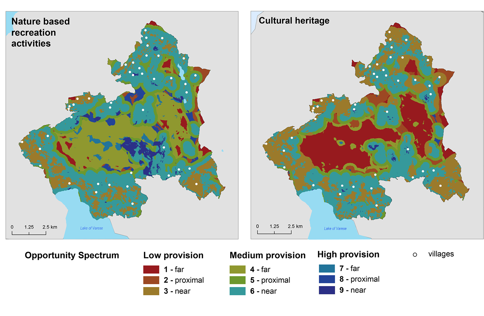
Mapping cultural ecosystem services (nature-based recreation activities and cultural heritage) based on mapping service provision versus access to the service. Service provision is expressed in three ordinal classes (low, medium and high) while access to the service is approximated by proximity (expressed in three ordinal classes: far, proximal, near). The case study relates to Campo dei Fiori, a regional park in Lombardy (Italy).
By using information on other values or by participatory mapping approaches (Chapter 5.6.2), the potential for ecosystems to provide a suite of cultural ES including education, inspiration or spiritual experiences can be mapped. In Figure
Conceptual questions
Even in the case of commonly mapped ES such as food, climate regulation or recreation, conceptual problems may obstruct the application of maps in policy and decision-making processes. What exactly to map is a recurring question. The ES cascade (see Chapter 2.3) may give guidance but invokes typical problems related to mapping as well. The cascade provides a logical and well-established framework to describe the flow of ecosystem goods and services from nature to society. It distinguishes between biophysical structures and processes, ecosystem functions, services, benefits and values.
Conceptual problems may, however, arise due to the fact that ES can be mapped along different elements of the cascade. Mostly, many provisioning ES are not mapped as contributions of ecosystems to human well-being but as the realised benefits or the final goods from ecosystems which are sold on markets (total harvested crops, livestock production, water abstracted, timber removals, fish yields etc.). However, these maps also contain the human energy input that is applied to harvest or extract these provisioning ES (Chapter 5.1). In managed systems, ecosystem structures, processes and functions (and resulting ES) are heavily modified by additional anthropogenic system inputs such as fertiliser, water, energy, technology, labour or knowledge, affecting especially regulating ES and biodiversity. In particular for crop production, these human-based inputs are far more important than the natural energy and matter inputs but it is difficult to separate and map these two components. It still needs to be tested whether a distinction between natural and anthropogenic contributions is feasible for quantification and mapping of ES, especially on larger spatial and temporal scales.
In contrast, ecosystem processes, structures or functions are mapped for many regulating ES. Regulating ES are, by nature, closely linked to biophysical structures and processes and functions. For some regulating ES, such as mediation of flows (including mass, liquid and gaseous flows) or maintenance of physical, chemical, biological conditions (including soil formation, pollination and water conditions), clear overlaps with ecosystem functions like nutrient or water cycling are obvious. In order to avoid double-counting (see Chapter 6.1), a clear distinction between ecosystem functions and services has to be made in case they are to be quantified, mapped, assessed and finally valued jointly. Even if many regulating ES are not (yet) perceived as services by society because they lack clear (direct) benefits or end-products, they need to be mapped and integrated in respective assessments. Otherwise regulating ES are in danger of being neglected in ecosystem assessments, especially when it comes to analyses of ES synergies and trade-offs.
Mapping demand for ecosystem services
Demands for many regulating ES are also not easy to define or to map (see example in Box 1). Demands and preferences for micro and regional climate regulation and related benefits can, for example, be highly individual and specific. Respective indicators often quantify temperature amplitudes or deviations of precipitation, wind or evapo-transpiration compared to surrounding areas or standard values. We are aware that regulating ES demands and related perceived human benefits may differ considerably.
For global climate regulation, ES benefits refer to non-desired temperature changes, storm events or coastal hazards. The service providing areas SPA (for example, the large forest belts) can be mapped at specific locations, whereas the service benefitting areas SBA (Chapter 5.2) are of global extension (see Figure
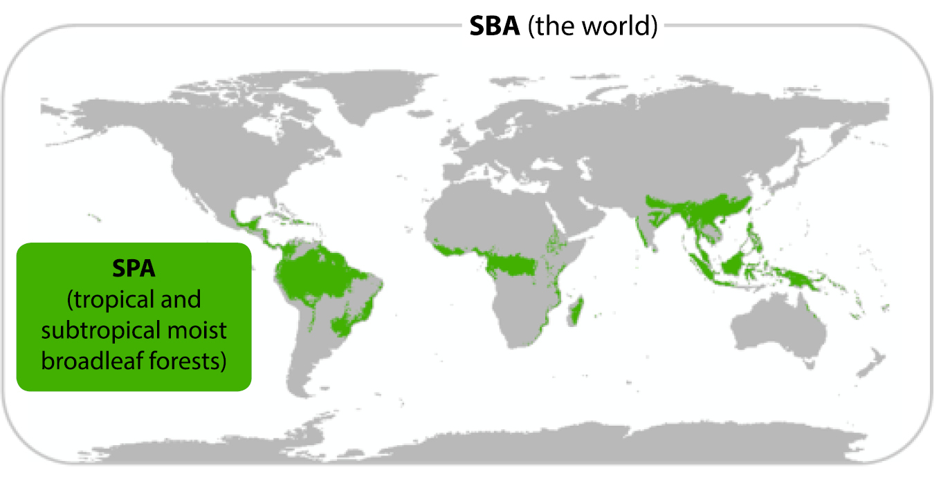
Example of global climate regulation with regional SPAs (service providing areas) and global SBAs (service benefiting areas).
Pollination and seed dispersal are very prominent examples of a regulating ES that is mapped frequently. The final goods would be the fruit or flower to be consumed or enjoyed by humans, whereas the pollination process itself (the pollen-transfer) could be seen as an ecosystem function or intermediate ES (Chapter 2.3), providing the base for the actual ES supply.
In order to map pollination, often potential habitats for pollinators, species numbers or the amount of pollinators are used as proxies to indicate the actual pollination function (see also Chapter 6.3). However, we need to be aware that habitats or the occurrence of certain species belong to biophysical structures and processes within the ES cascade (Chapter 2.3). Demand for pollination services can be mapped based on the amount and location of agricultural, garden or wild plants demanding pollination.

For provisioning ES demand-mapping, the problem of often highly complex and globalised supply-demand patterns occurs for many goods and services. For goods that are based on multiple ES (e.g. a chair made of wood, fabric, metal), the question arises where to localise the demand for the particular services and where to map their supply. A solution can be to consider the place of the last contribution of an ecosystem as the place of supply (e.g. the forest) and the place of final use by the consumer (sitting on a chair) as the demand area or SBA. Complex trading schemes of goods, which involve several retailers, resellers and distributors along the path from the ecosystem to the final consumer are adding to the issues of mapping provisioning ES supply-demand patterns.
For many cultural ES, the question about whether the benefits contributing to individual well-being should be located i) directly at the place where the service is provided (e.g. a SPA in the form of a good beach used for recreational activities), ii) at the home of the beneficiary (i.e. the place where she/he spends most time of the year), or iii) at both sites. All three options make sense but are related to uncertainties and may lead to misinterpretations.
Spatial or temporal questions
A single map has two spatial dimensions and is static, so it is not very useful to show temporal changes. Yet, the environment and ecosystems exist in three dimensions in space and often undergo highly dynamic changes (fourth dimension). This contrast brings about particular challenges for mapping which we illustrate here for certain ecosystems and their services.
Most ecosystems can be relatively well mapped and spatially separated. Forests, grasslands or wetlands obviously occur in three dimensions but it is relatively straightforward to map them and assign specific ES to them. Often ecological processes in terrestrial ecosystems follow seasonal cycles related to primary production so that annual averages can be calculated and attributed to these ecosystems and, hence, to ES maps (Chapter 5.3).
Marine areas are more complex to map due to their three-dimensionality, water current dynamics (especially in tide-influenced waters) and the significantly different components they include. One solution could be to produce ES maps per ecosystem type and per service: one for the water surface (relevant, for example, for cultural ES, transport, energy), another for the water column (e.g. for nutrition, energy, mediation of flows, maintenance of physical, chemical, biological conditions) and one for the benthic habitats and the sea bottom (e.g. materials, nutrition, mediation of flows).
Groundwater represents a special case as it challenges both the representation of ecosystems in maps (often based on land cover data) and the typical classification systems for ES. Groundwater ecosystems are vital providers of water for drinking and non-drinking purposes. In two dimensions, they spatially overlap with all other ecosystems and processes in groundwater layers sometimes take place in decades, if not longer. Several questions emerge with respect to groundwater as an ES: which ecosystems are the providers of groundwater ES, where to localise the supply and to what extent is the provision of groundwater for drinking or non-drinking purposes an "ecosystem" service (see Box 2 for further details)?
The easiest and most pragmatic approach is to assign the groundwater ES to the ecosystems or land cover types lying above the ground.
There is also an ecological rationale for doing so. The generation of groundwater ES is mediated by ecological processes which take place in forests or agricultural ecosystems where vegetation influences the re-charge of groundwater layers beneath them. In addition, part of the groundwater is in the root zone of these ecosystems whereas other, deeper, groundwater layers are part of the abiotic crust of the earth. These aquifers also often receive groundwater from above but are mainly abiotic depositories of groundwater generated elsewhere (in spite of the presence of some biotic organisms). Above-ground, water supply based on groundwater only often occurs as discrete local phenomena such as springs, dwells or water taps. Transportation installations such as water pipes or canals lead to a spatial decoupling of SPAs and SBAs (Chapter 5.2).
A second approach considers groundwater as a separate ecosystem and accounts for the specific ES delivered by groundwater. Groundwater abstraction for different user purposes is assigned to this ecosystem type and not to the above-ground ecosystem where the abstraction takes place but this involves working with multiple maps to avoid overlap.
A third approach considers groundwater as a subsoil asset or as system which delivers abiotic flows.
It is difficult indeed to always identify a clear boundary between the abiotic and ecosystem components of natural capital. Water which also comes through in the treatment of groundwater in different related pilot studies is a key example in this regard. A guiding question for classifying natural capital components into abiotic or ecosystem elements needs to address whether or not a given component is primarily shaped or maintained by biological organisms and their interaction with the abiotic environment.
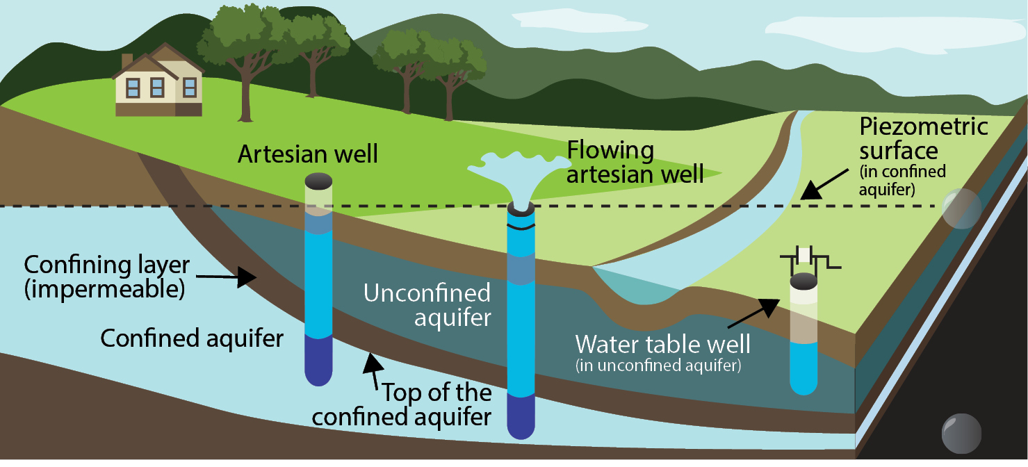
Example provisioning ES water supply based on groundwater or surface water (based on http://groundwater.sdsu.edu/).
A similar question can be addressed when considering soil and soil-related ES. Soil is an important part of our natural capital and soil science is a well-developed discipline with a great deal of information available in soil maps. Prominent ES delivered by the soil are erosion control and, obviously, soil formation and composition. The first two approaches also apply here when accounting for soil ES: either they are assigned to the ecosystem they support (e.g. forest, cropland, or grassland) or they are considered as a separate soil system overlapping with other ecosystems. Both approaches are possible depending on the context and the purpose of the study.
Technical questions
Available data, indicators and maps of ES come with different spatial extent and resolution. Examples of these include: forest inventories may use coordinates to report on forest standing plots; model-based observations on the regulation of water quantity and quality are often organised according to hydrological units; crop statistics are reported for parcels or using political boundaries. Integrated ES assessments often require bringing these different data sources and maps into a single, standardised format, for instance a 1 km? grid or polygons representing municipalities or regions. This requires the use of GIS functions such as up- and downscaling or zonal averaging. These operations may be a source of statistical bias that can seriously affect the results, also referred to as the Modifiable Areal Unit Problem (MAUP; see Chapter 3.1 and 6.1).
Summary tables
The following tables give an overview of selected ES, common mapping problems with them and suggested solutions.
Selected regulating ecosystem services (ES), mapping problems and suggested solutions.
| Regulating ES examples | Possible problems | Solutions |
| Global climate regulation | Focus on carbon dioxide and climate change only | Integrative mapping approaches (Chapter 5.6) |
| Focus on carbon sequestration only | Combination of carbon sequestration and storage (i.e. in soils) | |
| Large difference between SPA and SBA | Overlay or intersect SBA and SPA maps (Chapter 5.2) | |
| Regional climate regulation | ES demand relates to certain human preferences of ecosystem states | Relate to standard, critical or legitimate values |
| Ventilation and transpiration | Human preferences or defined (critical) levels | |
| Hydrological cycle and water flow maintenance | Human preferences of "constant water flow" (flood and drought prevention) | Combine with respective ES demand maps |
| Soil formation and composition | Soil formation is a very slow process | Consider long-term effects (Chapter 5.3) |
| Strong overlaps with ecosystem functions | Distinguish between natural processes, external inputs and avoid double-counting | |
| Mass flow regulation (e.g. erosion control) | Avoided events need be assessed | Model-based approach with and without ES supplied (Chapter 4.4) |
| Flood or storm protection | ||
| Pollination | Strong overlaps with ecosystem functions, high potential of double-counting | Separate between potential use and actual use (see Chapter 5.1) Little concern about double-counting when mapping single ES |
| Pest and disease control | ||
| Mediation of waste, toxics and other nuisances | ||
| Maintaining water conditions |
Selected provisioning ecosystem services (ES), mapping problems and suggested solutions.
| Provisioning ES examples | Problem | Solution |
| Cultivated crops, reared animals, aquaculture | High impact of external anthropogenic system inputs | If possible, include indicators of human contributions and external environmental effects |
| Complex ES supply chains | In absence of better data, use spatially explicit crop and stock statistics for mapping | |
| Animal stables and aquafarms = locally discrete point SPA |
||
| Biomass-based energy sources | E.g. maize, rape: final use not always clear | Combination with respective ES demand |
| Timber | Temporal: long growth phases | Distinction between ES potential and flow (Chapter 5.1) |
| Groundwater for drinking/ non-drinking purposes |
Subsurface SPAs; SBAs delocalised and point sources (wells, pipes) | See Box 2 in this chapter |
Selected cultural ecosystem services (ES), mapping problems and suggested solutions.
| Cultural ES examples | Problem | Solution |
| Physical and experiential interactions | Different and subjective preferences | Participatory GIS (Chapter 5.6.2), Citizen science (Chapter 5.6.3) |
| Intellectual and representative interactions | ES supply and demand difficult to indicate, quantify and localise | Applying the ROS approach (see this Chapter) can help raising awareness Participatory GIS (Chapter 5.6.2) |
| Spiritual and/or emblematic interactions |
Solutions
Although not all ES can readily be mapped, we still argue that an inclusive approach is to be preferred. Too often, ecosystem assessments focus on selected ES only such as food production, climate regulation, or water quality regulation using lack of knowledge, data gaps and conceptual problems as an argument for justifying a limited perspective.
However, the strength of ES as a concept is that it offers scientists, planners and decision-makers a frame that encompasses all benefits we receive from nature. We should therefore act accordingly. The ES matrix approach (see Chapter 5.6.4) is a first valid alternative to map and assess problematic ES and put them in the whole picture. The combination of using land use and land cover data and expert- or evidence-based ranking of potential supply and demand as proxies has been successfully applied at various spatial scales and for different purposes. Several chapters of this book provide more detail or use matrix-mapping for different applications.
For cultural ES, we advance here the approach based on mapping nature-based recreation. Mapping cultural ES inevitably depends on quantifying an information flow from nature to people. Mapping the recreational opportunity spectrum involves combining ecological data with socio-economic information such as demographic statistics and the location of infrastructure and can serve as an example for mapping other cultural ES.
More efforts could be applied to the use of biodiversity data for mapping ES. A recent study used species occurrence data from GBIF, the global biodiversity information facility, to map wild food in Europe. Species are the basis of ecosystems and thus the main service providing units for several ES (see also Chapter 2.2). Linking occurrence data with trait information will be key to mapping those ES with a strong connection to biodiversity such as pollination.
Importantly, high resolution mapping is a solution to several conceptual and technical problems. This is particularly evident in heterogeneous landscapes with a mixture of cropland, semi-natural vegetation and forest.
Quantifying ES such as food production, pollination, or maintenance of soil quality often leads to questions about double-counting. This arises as a result of the latter two regulating ES contributing to the former service. A detailed mapping of cropland with spatial delineation of the semi-natural vegetation such as hedges, forest patches and grass strips also allows spatially segregating areas that provide regulating ES from areas that are dedicated to production. Moreover, double-counting mainly occurs when different ecosystem functions, services and benefits are finally aggregated to one single number (such as the total economic value TEV). Compiling maps of individual ES helps to avoid double-counting and highlights the vital role of regulating services and ecosystem structures.
Further reading
- Burkhard B, Kandziora M, Hou Y, Muller F (2014) Ecosystem Service Potentials, Flows and Demands - Concepts for Spa- tial Localisation, Indication and Quanti- fication. Landscape Online 34: 1-32.
- Crossman ND, Burkhard B, Nedkov S, Wil- lemen L, Petz K, Palomo I, Drakou EG, Martin-Lopez B, McPhearson T, Boyano- va K, Alkemade R, Egoh B, Dunbar M, Maes J (2013) A blueprint for mapping and modelling ecosystem services. Eco- system Services 4: 4-14.
- Grizzetti B, Lanzanova D, Liquete C, Reynaud A, Rankinen K, Hellsten S, Forsius M, Cardoso AC (2015) Cook-book for water ecosystem service assessment and valuation. EUR 27141. Publications office of the European Union, Luxembourg.
- Haines-Young R, Potschin M (2010) The links between biodiversity ecosystem services and human well-being. In: Raf- faelli D, Frid C (Eds) Ecosystem Ecology: A New Synthesis. Cambridge University Press, Cambridge, 110-139.
- Martinez-Harms MJ, Balvanera P (2012) Methods for mapping ecosystem service supply: a review. International Journal of Biodiversity Science, Ecosystem Services & Management 8: 17-25.
- Villamagna AM, Angermeier PL, Bennet EM (2013) Capacity, pressure, demand, and flow: A conceptual framework for analysing ecosystem service provision and delivery. Ecological Complexity 15: 114-121.
- Paracchini ML, Zulian G, Kopperoinen L, Maes J, Schagner JP, Termansen M, Zandersen M, Perez-Soba M, Scholefield PA, Bidoglio G (2014) Mapping cultural ecosystem services: A framework to assess the potential for outdoor recreation across the EU. Ecological Indicators 45: 371-385.
- Schulp CJE, Thuiller W, Verburg PH (2014) Wild food in Europe: A synthesis of knowledge and data of terrestrial wild food as an ecosystem service. Ecological Economics 105: 292-305.
6.3. Uncertainty measures and maps
Introduction
Many ecosystem services (ES) are very difficult or even impossible to measure. While the amount of crops produced is monitored at a detailed level in the EU, it is less straightforward to quantify how many potential floods have been avoided and to what extent functioning of the ecosystem renders this flood risk mitigation. Consequently, ES are commonly mapped based on a combination of a limited number of measurements, expert-based or empirically derived proxies and model-based mapping procedures. For example, the capacity of the landscape to sequester CO2 has been mapped through first measuring CO2 sequestration rates in different ecosystems, which are then upscaled by combining average sequestration rates per ecosystem with a map delineating these ecosystems.
In these modelling or upscaling approaches, as well as in the underlying measurements, uncertainties arise. First, measurement equipment is not 100 % accurate and people who measure environmental variables can make mistakes. A common method to measure soil organic carbon stocks clearly illustrates this situation. In the "loss on ignition" method, a soil sample is first dried in an oven to remove all soil moisture and then weighed. Next, the sample is placed in an oven at over 400 °C for 24 hours to burn all organic matter. The sample is then weighed again and the weight difference represents the amount of organic matter. This is translated into organic carbon using a conversion factor of (1/1.72) g carbon per g organic matter. Both weighing procedures have a small error, resulting in an uncertainty in the amount of organic matter. The conversion factor from organic matter to organic carbon is well established, but differs depending on the origin of the organic matter, meaning that the factor is uncertain as well. Altogether, the loss on ignition method has an uncertainty of approximately 2 %, meaning that, when a soil organic carbon stock of 5 % is reported, the value can actually vary between 3 % and 7 %.
In many approaches for mapping ES, such measurements are then coupled to maps of land cover or environmental variables such as soil maps or elevation maps to create an ecosystem service map. Land cover maps are commonly derived from remote sensing imageries. These maps are uncertain with regard to the location or shape of objects and with regard to the characteristics of mapped objects. Uncertainty on the shape or location of objects is called geometric uncertainty and is a result of the spatial resolution of the data. While high-resolution remote sensing imagery such as the 20 m SENTINEL products are able to capture small land cover patches and land cover types with a limited cover, upon a coarser resolution, such features get lost. Neither linear landscape elements like hedgerows, ditches and tree lines nor individual trees can be captured even with a 20 m resolution. For several ES, such landscape elements are essential for the supply, meaning that the inability to capture them limits the possibility of satellite-derived land cover data in mapping ES.
Uncertainty on the attribute values is called thematic uncertainty and arises when classifying the reflectance signature into a land cover classification. Thematic uncertainty implies that when a land cover map displays grassland, there is, for example, a 90 % probability that there is actually grassland on that specific location while there is a 10 % probability that, in reality, another land cover type is present.
Mapping of other biophysical variables which are used as input to ecosystem service maps exhibit additional uncertainties due to upscaling of measurements. This includes simplifying the continuous variation of soil characteristics into soil types, or inaccuracies in measuring elevation. An additional source of uncertainty for mapping ES is that, due to data availability limitations, inputs from a range of different years are often used.
Additional to these "technical" uncertainties, conceptual uncertainties may arise as well. Most ES can be defined in different ways. This is related to the understanding of the processes that ensure the service supply and to the aims of the mapping study.
When mapping an ecosystem service, many different choices can be made on the indicator used, the data and methods used to quantify the indicator and the final presentation of the indicator. When a set of maps and measurements, each with an uncertainty range as a result of these technical and conceptual limitations, is combined into an ecosystem service map, the uncertainties in the input propagate into uncertainty of output in ecosystem service maps.
Uncertainties in large-scale ecosystem service maps: pollination as an example
On a global scale, the production of 35 % of the food crops depends on pollinators. Both managed honeybees as well as wild bees are important for pollination. Several crops are exclusively pollinated by wild pollinators while, for many other crops, wild pollinators significantly contribute to the yield quantity and quality. This is a frequently mapped ecosystem service and the approaches available for mapping clearly demonstrate the source and impact of conceptual and technical uncertainties that arise when mapping ES in general.
Mapping an ecosystem service basically involves, firstly, selecting an indicator to quantify the service; next gathering spatial and non-spatial input data in an iterative manner along with defining the model to quantify the service; and finally, applying the model to the data.
Each step introduces specific uncertainties.
Indicator selection
The ecosystem service "pollination" can be quantified using different indicators (Table
Overview of indicators for the ecosystem service "pollination".
| Category | Definition |
| Landscape-based indicators | Capacity of the landscape to support pollinator communities |
| Percentage area of potential pollinator habitat | |
| Distance to pollinator habitat | |
| Probability that a location is visited by pollinators | |
| Species-based indicators | Abundance of pollinators |
| Abundance of specific pollinator species | |
| Species richness of pollinators | |
| Crop-based indicators | Yield quantity |
| Financial benefits of yield of pollinator-dependent crops | |
| Percentage yield loss upon absence of pollinators |
Which indicator to choose depends on the scale and aim of the study. For a detailed, small-scale study that aims to assist with the planning of green infrastructure in a specific agricultural landscape, it may be relevant to consider which crops are typically grown in the landscape, which pollinators are important to those crops and what are the additional habitat requirements for those species. Here, indicators based on species composition or on abundance might be the most appropriate. ES are often mapped on a national or continental scale to support national or EU policies. At such a large scale, abundance is often not feasible due to lack of data to calibrate or validate the required models and the variation in space and time of crops grown makes it less relevant to distinguish specific pollinator guilds. Therefore, more generic measures such as landscape composition are used. Several large-scale pollination maps are based on the presence of suitable habitat for pollinators and the distance to these habitats in croplands.
Data selection
After choosing an indicator for quantifying the ecosystem service, input data for mapping should be selected and a model for calculation needs to be defined. A pollination indicator which is based on landscape composition, commonly uses land cover data as input data. For most parts of the world, a few different land cover maps are at least available. For example, the Netherlands is covered by global-scale MODIS products and digital elevation models, the European scale CORINE land cover (CLC) and the Dutch LGN (land use). Each of these maps has an uncertainty associated with it and different maps differ in thematic detail and spatial resolution and in accuracy. The most accurate land use map of the Netherlands (LGN) has a classification accuracy of 85-90 %, while the CLC has an accuracy of 80 % and the global scale GLC2000 of 68 %. Apart from the uncertainty within the maps, the maps also differ in representation of the landscape. For example, an area with > 15 % tree cover is considered a forest in GLC2000 while in CLC a 30 % threshold is used to distinguish forests among other land cover types. Some of the land cover maps include a few details on land use by, for example, distinguishing pastures from natural grasslands. Thus, the choice of a specific land cover map for mapping an ecosystem service to a certain extent defines the output.
Model definition
A key parameter for pollination services is the distance between a pollinator habitat (nesting site) and the crop which needs pollination. For calculating the distance to pollinator habitat using a land cover map, one should decide whether each land cover type provides habitat or not. This introduces new uncertainties. While for many individual pollinator species, habitat requirements are known, these often do not match the level of detail displayed in land cover maps. One can only assume that the specific vegetation type and structure or host plant which a pollinator community requires, is present in a land cover type that is only described with a level of detail like "natural grassland" or "deciduous forest". Secondly, a single land cover type can include both suitable and unsuitable areas, dependent on the types of vegetation included in the land cover or dependent on the management. Based on the knowledge of pollinator behaviour and of the land cover map, the map maker has to distinguish between presence or absence of a habitat. Depending on background knowledge and the exact nature of the uncertainties described above, different map makers can decide differently in similar situations. This introduces a new uncertainty.
More uncertainty arises when calculating the distance to habitat, depending on the resolution of the data. Each pixel gets assigned one distance value which, especially when using coarse resolution data, can deviate. In addition, land cover data often fail to properly represent small landscape elements such as tree lines, hedgerows or individual trees. An alternative approach that can help overcome this is, for example, using a map of the density of such elements. But deriving distance to habitat from a density map also introduces a new uncertainty.
Relations between distance to habitat and the effectiveness of animal pollination have been previously established. Close to natural habitat, bee abundance and species richness tend to be high while richness and abundance decrease upon increasing distance to habitat. While this general principle is well known, in different situations the decrease of pollinator abundance or theoretical visitation rates can be hugely different. Figure
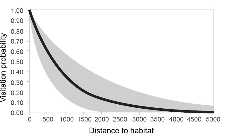
Relation between distance to pollinator habitat and probability that a location is visited by pollinators. The black line is an average value for temperate regions while the uncertainty range is indicated in grey. Based on (
The impacts of input data uncertainty on the output uncertainty are demonstrated in Figure

Impact of input data on mapping ecosystem structure and function. For distance to nature (left) and percentage yield reduction as a function of distance to nature, maps based on four EU / global scale maps were compared with a detailed reference map (based on
Figure

Dealing with uncertainties
As ecosystem service mapping will always involve uncertainties, it is important to deal with these uncertainties in the best possible way. Dealing with uncertainties in ecosystem service maps means (1) improve methods for ecosystem service maps so as to reduce uncertainties to the largest extent possible; (2) quantify and communicate uncertainties and (3) account for uncertainties when using ecosystem service maps in policy and practice.
Improving measurements
Firstly, for several ES, there is a lack of clarity about how to define the service, a lack of process understanding and a limited measuring accuracy. In all of these three sources of uncertainty, there is scope for improvement. For each case of mapping, it should be carefully decided how a service can be best quantified. Furthermore, for several ecosystem service models, the underlying measurements can be expanded and better stratified. Process understanding for some services needs to be better underpinned by field studies.
Quantifying uncertainties
Regardless of the scope for improvement of ecosystem service models, it is important to realise that uncertainties in ecosystem service maps cannot be completely ruled out. Sensors will never be 100 % accurate and the provision of ES is a complex and multifaceted process where multiple datasets have to be combined, always involving some kind of expert judgement. It is, therefore, important to be transparent on uncertainties in ecosystem service maps. If ES are mapped using complex process-based models (Tier 3 approaches; see Chapter 5.6.1), an uncertainty analysis or a Monte Carlo approach can be used. In a Monte Carlo approach, the indicator is calculated several thousand times. Each time, actual input values for calculation are drawn from a probability distribution of each input, resulting in different but realistic representations of the indicator. From these different representations, an average value of ecosystem service provision can be calculated, as well as indicators that quantify the uncertainty, such as a probability range, a standard deviation, or a probability that a specific target or threshold value is met or not.
A simpler uncertainty analysis includes making an inventory of the range of each input. Next, for each input, one should identify if it increases or decreases provision of the service. Finally, the ecosystem service map should be calculated with the combination of inputs that provides a minimum, a maximum and an average indicator value. This provides the possible range of the indicator.
For methods that completely rely on expert judgement (Tier 1 approaches; see Chapter 5.6.1), it is important not to rely on a single expert, but instead to take stock of a wider range of expert knowledge in the field. Ratings by different experts on the capacity of the landscape to supply ES can, for example, be translated into a measure for the "agreement" of different experts and, with that, provide an indicator for the uncertainty.
Intermediate approaches that combine expert knowledge with additional data or simplify process-based models (Tier 2 approaches; see Chapter 5.6.1) can use an intermediate approach for uncertainty quantification as well. Bayesian Belief Networks, as discussed in chapter 4.5, are typical examples of models that can account for a broad range of uncertainty types and can assess the effects of these uncertainties on model outputs.
Dealing with uncertain maps
At the same time, scientists and policy makers use maps of ES on which to base analyses and decisions. Such decisions should be robust, meaning that they should not work out differently from what they are supposed to, because of the uncertainties in the maps. To ensure that uncertainties in ecosystem service maps do not impede decision-making, they must be quantified and communicated by map makers. Here, an uncertainty analysis, as described above, is essential and clear reporting of uncertainties is compulsory.
On the other hand, policy makers and other users of ecosystem service maps should account for the level of certainty in their decision-making. To do so, a dialogue between policy makers and mappers is essential (Chapter 6.4) to ensure that the indicator mapped actually reflects the request by policy makers, given that the indicator is a major source of uncertainty. Users of ecosystem service maps should also be careful when making planning decisions based on ecosystem service maps. Also, for map users, it might be important to take stock of the broad knowledge in the field rather than relying on a single map upon decision-making. Finally, policy makers should be cautious upon using ecosystem service maps for decision-making.
Further reading
- Gret-Regamey A, Brunner SH, Altwegg J, Bebi P (2013) Facing uncertainty in ecosystem services-based resource management. Journal of Environmental Management 127: 145-154.
- Jacobs S, Burkhard B, Van Daele T, Staes J, Schneiders A (2015) The Matrix Reloaded: A review of expert knowledge use for mapping ecosystem services. Ecological Modelling 295: 21-30.
- Schulp CJE, Alkemade R (2011) Consequences of Uncertainty in Global-Scale Land Cover Maps for Mapping Ecosystem Functions: An Analysis of Pollination Efficiency. Remote Sensing 3: 2057-2075.
- Schulp CJE, Burkhard B, Maes J, Van Vliet J, Verburg PH (2014) Uncertainties in Ecosystem Service Maps: A Comparison on the European Scale. PLoS ONE 9: e109643.
- Schulp CJE, Lautenbach S, Verburg PH (2014) Quantifying and mapping ecosystem services: Demand and supply of pollination in the European Union. Ecological Indicators 36: 131-141.
- Stoll S, Frenzel M, Burkhard B, Adamescu M, Augustaitis A, Bae?ler C, Bonet FJ, Carranza ML, Cazacu C, Cosor GL, Diaz-Delgado R, Grandin U, Haase P, Hamalainen H, Loke R, Muller J, Stanisci A, Staszewski T, Muller F (2015) Assessment of ecosystem integrity and service gradients across Europe using the LTER Europe network. Ecological Modelling 295: 75-87.
- Ricketts TH, Regetz J, Steffan-Dewenter I, Cunningham SA, Kremen C, Bogdanski AK, Gemmill-Herren B, Greenleaf SS, Klein AM, Mayfield MM, Morandin LA, Ochieng A, Viana BF (2008) Landscape effects on crop pollination services: are there general patterns?, Ecology Letters 11(5): 499-515.
6.4. Map interpretation/end-user issues
Introduction
Maps are very powerful tools to communicate complex geographic information from the map-maker (the cartographer) to the end-user (such as a decision-maker). As in all communications, there are information losses and/or modifications during the transmission from the sender to the receiver. Ecosystem service maps are a specific case due to their high thematic complexity, adding further potential for (mis)interpretation of the intended messages. It is therefore essential that the end-users not only have access to the map, but are also aware of any interpretation issues such as the categorisation of ecosystem services (ES) used (Chapter 2.4), choice of spatial scales (Chapter 5.7) and uncertainties or scientific errors (Chapter 6).
Map communication model
Maps can usefully be understood as a form of visual communication to describe spatial phenomena and their relationships. In early understandings, building, for example, on the transmission model of communication put forward by Shannon and Weaver in 1949, maps were seen as media for spatial information sent from the mapper to the map-users (Fig.

Specifics of ecosystem service maps
Ecosystem service maps are complex as they reflect the level of difficulty we find ourselves in managing the environment and ensuring equitable benefits across society. The science underpinning the actual mapping of ES is still unresolved despite recent advances. The issue of mapping ES is further compounded by the need to bring together and display the supply of a service and its demand (including flow; see Chapter 5.1) using environmental, economic and societal factors, a difficult endeavour when working in conventional two-dimensional space (Chapter 3.7). With the concepts of ES and natural capital rising high up the political agenda through processes such as the Intergovernmental Platform for Biodiversity and Ecosystem Services (IPBES), CBD Aichi Target 14, the UN SDGs or the EU's Biodiversity Strategy, there is a need to ensure ecosystem service mapping is scientifically robust and easily understood (Chapter 7.1).
Particular challenges surrounding the communication of ES maps to end-users include:
- The existence of diverging categorisations (Chapter 2.4) and conceptualisations of ES (e.g. as potentials, flows or benefits of ecosystems; Chapter 5.1) requires clearly specifying the exact meaning of what is being illustrated on the maps. End-users may be aware of different categorisations and conceptualisations of ES but will not be aware of the associated interpretation issues.
- The possibility of spatial misfit between the areas that supply ES and the areas in which the benefits are consumed (Chapter 5.2). Communicating the choice of spatial scale or the mismatch between supply and beneficiaries can conceptually be difficult to understand.
- The complicated spatial overlap of the provisioning and/or benefitting areas concerning several ES at the same site. Communicating this overlap spatially on maps can build upon, for example, hotspot and cold-spot analyses (Chapter 5.7).
- The difficulty to communicate the uncertainties inherent in the delineation, quantification and evaluation of ES provision, supply and benefits despite the connotation conveyed by maps as authoritative spatial information (Chapter 6.3).
Ecosystem service map-makers
In recent years, ecosystem service mapping has gained prominence as a scientific field and as an output from research. It has permitted different disciplines (such as ecology, economics and social sciences) to analyse different types of information together, often resulting in highly complex and specialised maps.
With the advent of desktop Geographic Information Systems (GIS) and a number of ecosystem service mapping tools (see Chapter 3.4), creating maps has become easier and seemingly without the requirement of having specific cartography training. However, the ease at which ecosystem service maps nowadays can be created needs to be balanced with the danger of creating a badly designed map. Maps that are not well designed or lack cartographic logic (Chapter 3) increase the risk of misinterpretation by decision-makers or even the deliberate abuse of ecosystem service information in non-sustainable environmental resource management. Therefore, (at least basic) cartography training and knowledge are necessary in order to avoid typical technical and thematic pitfalls of map-making.
Ecosystem service map end-users
The end-users of ecosystem service mapping products vary in nature and in their purpose for wanting a map. End-users could be:
- Decision-makers working at different scales who wish to make a specific land-use decision such as approval for a dam, road or land use change (e.g. forest to agriculture; see Chapter 7). The types of questions which are asked are highlighted in Table
1 ; - A decision-maker or NGO wanting to engage a group of stakeholders or the public in a specific issue such as demonstrating their links and benefits obtained from a particular site;
- A practitioner synthesising information to present to a decision maker around a specific issue;
- Policy makers on different levels wanting to illustrate progress towards certain policy goals;
- The scientific community, students and teachers.
Example of policy questions from the EU that ecosystem service mapping might address (adapted from
| Policy questions | Policy & research actions |
| What are the status and trends of the EU's ecosystems and the services they provide to society? | Biophysical mapping of ES using data and models. |
| What are the drivers causing changes in the EU's ecosystems and their services? | |
| How might ecosystems and their services change in the EU under plausible future scenarios? | Mapping and valuation of ES as part of an integrated and stakeholder-based approach to sustainable land management and use of natural resources. |
| How can we secure and improve the continued delivery of ES? | |
| Can we set priorities for ecosystem restoration within a strategic framework at sub-national, national and EU level? | |
| Can we define where to strategically deploy green infrastructure in the EU in urban and rural areas to improve ecosystem resilience and habitat connectivity and to enhance the delivery of ES at member state and sub-national level? | |
| How can we foster synergies between existing and planned initiatives at local, regional or national levels in member states, as well as how to promote further investments, thereby providing added value to member states action? |
Although all these user groups may find ecosystem service maps useful, once again the risk of misinterpretation is high. Many of the individuals involved will often not have a specific cartography education needed to 'read' and understand a map. Moreover, the map may be only one piece of evidence that their decision-making is based on.
Sources of uncertainty in map interpretation
Even if the best data, best model or best available methods have been used by a very skilled map-maker, the applicability of a map can be hampered by limited map reading/interpretation skills of the actual map end-user. Maps are generalising models of reality (Chapter 3.2) with inherent uncertainties related to all steps of map production. Lack of expert knowledge concerning ecosystem service supply and demand schemes can cause map misinterpretations. Much of the information included in ES maps is very complex and the information is highly aggregated to be directly used in practical applications. On the other hand, even a highly trained map-user with comprehensive expert knowledge cannot overcome weaknesses in data and map compilation.
In particular, the challenges can be summarised as providing maps:
- at the scale appropriate for planning and management,
- at the right point in time to make informed decisions,
- in an accessible manner and
- in communication formats appropriate for diverse user groups.
Solutions
In recent years there has been a call from the end-user community for more scientific outputs to be policy-relevant and for the co-development of outputs. However, policy-relevance and scientific integrity need to be balanced accordingly. Therefore the question is: how do you create a fit-for-purpose map that is scientifically robust? The first solution is to improve the communication between the map-maker and the end-user. Secondly, there is a need to improve the transparency of how the map was created and the uncertainties embedded in the map. Lastly, the reproducibility and the comprehension of the results need to be improved (e.g. better maps produced).
Engaging the end-user before the map is developed will allow the map-maker to understand how the map is going to be used, i.e. what question will the map be used to answer (Chapters 4.6 and 5.4)? The map- maker can then use this information to determine the degree of precision required, as it is not always necessary to use the highest data resolution with the most complex methods (Chapter 5.6.1). Often, simpler easy-to-comprehend approaches (Chapters 4.6 and 5.6.4) may deliver results that are easier to communicate.
The scientific community is also required to continuously improve the methods that are used to quantify, measure, monitor, model, map and value ES. These methods should not only be accepted by their peers but also be communicated clearly to those practitioners who are frequently generating maps or interpreting maps for different decision-making contexts.
While the most desired outcome would be to have the user-community trained to understand spatial information generally and, more specifically, the interpretation of ecosystem service maps, this is not really feasible due to the high resources required. However, the user-community's capacity can be continually enhanced over the long-term through dialogues with scientists and practitioners.
Further reading
- Dent Borden D (1985) Principles of Thematic Map Design. Addison-Wesley Publishing. Reading, Mass.
- Hou Y, Burkhard B, Muller F (2013) Uncertainties in landscape analysis and ecosystem service assessment. Journal of Environmental Management 127: 117-131.
- Maes J, Egoh B, Willemen L, Liquete C, Vihervaara P, Schagner JP, Grissetti B, Drakou EG, La Notte A, Zulian G, Bouraoui F, Paracchini ML, Braat L, Bidoglio G (2012) Mapping ecosystem services for policy support and decision-making in the European Union. Ecosystem Services 1: 31-39.
- Monmonier M (1996) How to lie with maps. 2nd ed. The University of Chicago Press.
- Muehrcke PC (2005) Map Use: Reading, Analysis, and Interpretation. 5th ed. J P Pubns.
- Wood D, Fels J, Krygier J (2010) Rethinking the Power of Maps. Guilford Pubn.
Chapter 7. Application of ecosystem services maps
7.1. Mapping ecosystem services in national and supra-national policy making
Introduction
Despite the global efforts taken to conserve biodiversity it was clear in 2010 that the global ''2010 target'' of preventing the loss of biodiversity had not been met. The Millennium Ecosystem Assessment, the various subsequent sub-global assessments and The Economics of Ecosystems and Biodiversity study have increased awareness of the negative impacts of biodiversity loss on human welfare by addressing the value of ecosystems and biodiversity for sustaining livelihoods, economies and human wellbeing. Failing to incorporate the values of ecosystem services (ES) and biodiversity into economic decision-making has resulted in investments and activities that degrade natural capital.
In 2010, the tenth meeting of the Conference of Parties (COP 10) to the Convention on Biological Diversity (CBD) led to the adoption of a global Strategic Plan for biodiversity for the period 2011-2020. The ''2020 Aichi targets'' complement the previous conservation-based biodiversity targets with the addition of ES.
Anticipating the COP10, the European Union (EU) adopted a communication on "Options for an EU vision and target for biodiversity beyond 2010". For the first time, explicit reference was made to the practice of mapping ES in a high level policy document. Maps of ES were expected to help define the scope of the maintenance and restoration efforts needed to achieve the new biodiversity targets. Eventually, the mapping of ES was retained in the EU Biodiversity Strategy to 2020 as one of 20 actions to be implemented by the EU member states.
Well before 2010, South Africa had already pioneered ES research including mapping to support policy on biodiversity, restoration and poverty reduction. Thus, this chapter will start with the achievements in that country to illustrate how mapping can contribute to policy support or, vice versa, how mapping entered into various policies. In later sections, developments on mapping for policy in other parts of the world will be presented.
Mainstreaming ecosystem services into policy: South Africa
When the concept of ES came into the limelight in the mid to late 1990s, South Africa was one of the first countries to embrace it. In 1995, South African scientists carried out a ground-breaking study showing that invasive alien plants had a negative impact on water supply. The results were communicated to the then Minister of Water Affairs (Mr Kader Asmal) who later established a very successful Working for Water (WfW) programme aimed at removing invasive alien plants to improve water quantity in rivers, conserve biodiversity and provide jobs for local people. The WfW programme was so popular, its budget grew from $5M to about $50M and created about 35,000 jobs in just 2 years. This success has inspired other programmes such as "working for wetlands". This example shows that the concept of ES can be a very powerful tool in developing policies that promote sustainable land use and improving the livelihoods for poor people.
South African scientists have written many influential papers on the mainstreaming of ES into policy, most of them inspired through their experience in the implementation of biodiversity plans in their country. These lessons were incorporated within a new grassland initiative (www.graslands.org) led by the South African National Biodiversity Institute in Pretoria (SANBI). As an implementation strategy within the programme, stakeholders, such as mining companies and the agricultural sector, were brought in as partners in order to help them understand the value of ES in their business, how they can practise sustainable land use and minimise cost. The grassland programme was a huge success as stakeholders were able to directly see the benefits of conservation through the lens of ES.
Since the grassland programme, much progress has been made in integrating ES into policy and practice. In 2013, the Department of Environmental Affairs (DEA) in South Africa set up the GREEN FUND (GF) to support green economy initiatives. As examples, this GF has supported the service of climate regulation through low-carbon initiatives such as the planting of trees in Durban and a study of the importance of ecological infrastructure in delivering ES. Scientists in South Africa are investigating the use of ES as a key entry point into developing the Strategic Environmental Assessment (SEA) for Thekwini municipality. The SEA is a key policy instrument in guiding development plans for the city of Durban. ES have direct links to the well-being of people living in the city and are attractive to policy makers. These examples show that ES are being integrated into the national, regional and local policy and practice.
Mapping and Assessment of Ecosystems and their Services in the European Union (MAES) - A dedicated action of the EU Biodiversity Strategy
The mapping and assessment of ES is an essential part of the EU Biodiversity Strategy to 2020 and a necessary condition in making ES key parameters for informing about planning and development processes and decisions. In particular, Action 5 of the Strategy requires member states, with the assistance of the European Commission, to map and assess the state of ES in their national territory by 2014, assess the economic value of such services and promote the integration of these values into accounting and reporting systems at EU and national level by 2020.
The European working group on Mapping and Assessment of Ecosystems and their Services (MAES), which includes experts of the European Commission, the member states and the research community, has been instrumental in providing an analytical framework, a typology of ecosystems and ES and a first set of indicators for mapping and assessment. Importantly, the EU supports dedicated research under its framework programme for research (Horizon 2020) to support the member states of the EU with the implementation of this policy. The project (ESMERALDA), for example, provides detailed guidance to various stakeholders for mapping and assessing ES.
The work being carried out on the mapping and assessment of ecosystems and ES is not only important for the advancement of biodiversity objectives, including the development of Europe's green infrastructure, but also to provide information for the development and implementation of related policies on water, climate, agriculture, forest and regional planning.
Box 1 presents a special case on how the MAES initiative could profit from ongoing assessments in the frame of the EU's marine policy.
Under the present EU regulatory frameworks and the pressure to foster sustainable Blue Growth (COM(2012)494) in the marine regions of the EU, it is necessary to undertake more accurate, policy-driven research able to map marine ES. Competing uses of marine resources need to be analysed from a holistic perspective to enable achievement of the environmental goals and socio-economic needs that are often competing. ES maps are needed to provide information about the supply and demand of essential services in different coastal and marine regions. These services can be used by different sectors (such as fisheries or tourism and recreation) and supplied in variable scales: commercial fish are catches derived from large marine areas, while recreation destinations such as scenic and pristine beaches can be spatially quite restricted. Therefore, maps showing the marine hotspots of ES can be very useful for the EU Marine Spatial Planning Directive (MSPD; Directive 2014/89/EU) and should be disseminated to decision-makers, wider key stakeholders and the general public for both use and validation. Mapping of marine ES is a prerequisite for assessing ES and hence, for preparing environmentally and societal-relevant plans for usage of marine resources, i.e. maritime spatial plans. In the same manner, ES valuation can be used for estimation of the benefits of the EU Marine Strategy Framework Directive (MSFD; Directive 2008/56/EC) programme of measures when the target "good environmental status" is reached. Therefore the economic assessment that is a part of the MSFD assessment (in article 8 of the Directive 2008/56/EC) can directly provide information for the EU Biodiversity Strategy Action 5, should the ES approach be used in the assessment.
The MAES framework consists of 4 different process steps: 1) mapping the ecosystems, 2) assessment of the conditions of ecosystems, 3) assessing ES and 4) integrated assessment based on these three components (Figure
The current EU directives that govern the use and protection of marine environment, namely MSFD and WFD, together cover all marine waters (including transitional waters). MSFD, WFD and HD include assessment of ecological status and pressures and impacts that will provide information for the MAES process step 2 'assess the conditions of ecosystems'. MSFD and HD also provide data and information on the distribution of species and habitats for process step 1: mapping the ecosystems. MSPD can potentially provide data and information to assess the use of marine space and to derive indicators on demand of the ES for process step 3: assessing the ES. However, the data flow from the directives' reporting might still not be sufficient and additional environmental and socio-economic data could be needed to assess the supply of ES and to provide information for the MAES process step 4 'integrated ecosystem assessment'.
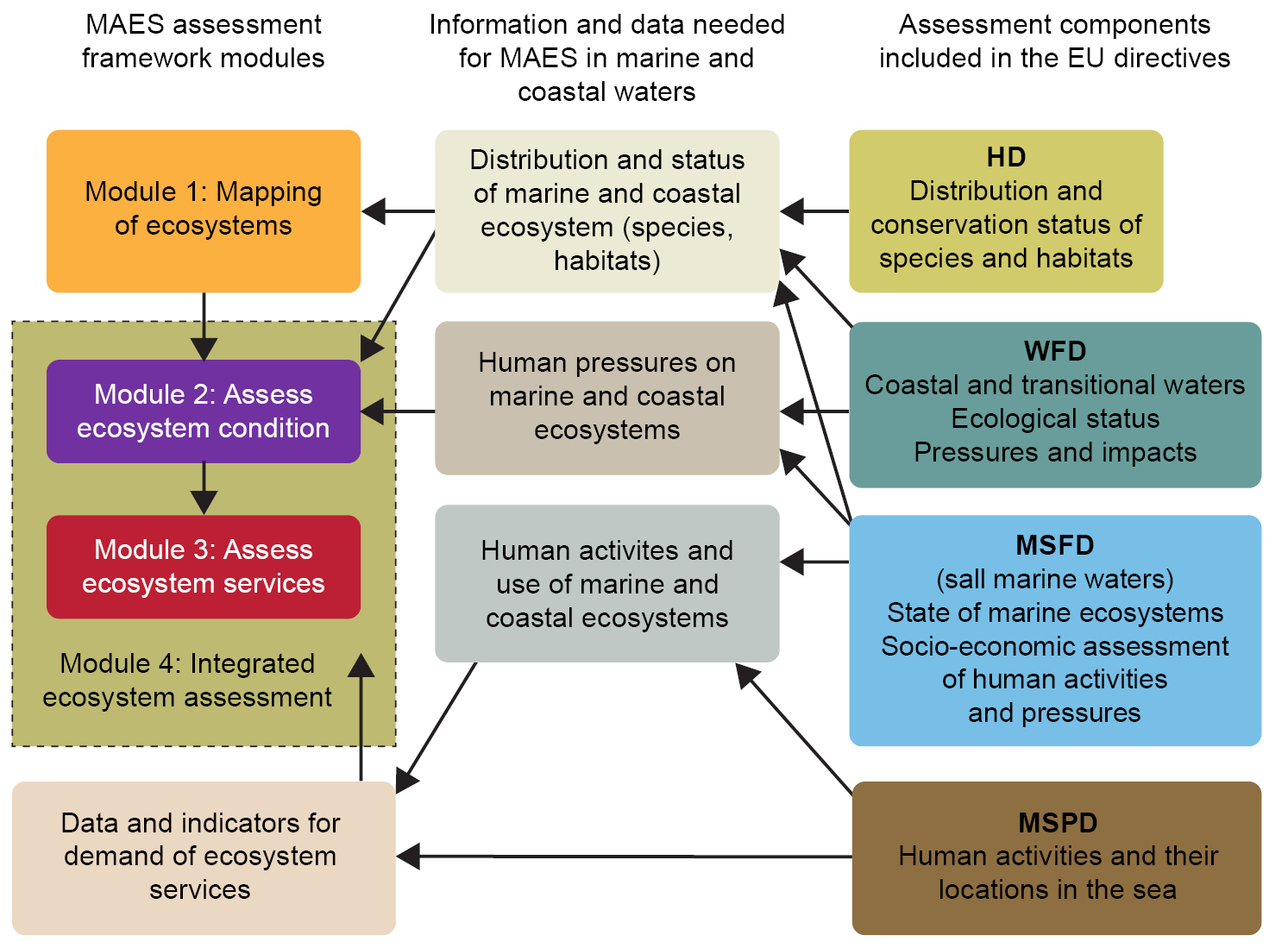
Overview of the linkages between the Mapping and Assessment of Ecosystems and their Services (MAES) framework and the EU directives that govern environmental status and biodiversity in marine and coastal areas: MSFD, WFD, the HD and the MSPD (see text for the explanations for the abbreviations). The linkages illustrate how the information and data from the assessments' components (from the implementation process of these directives) can feed into the MAES process and its modules 1-3. Optimally, such environmental and socio-economical flow of data could allow the use of the same information in multiple reporting purposes, if undertaken diligently.
China: A unique opportunity to mainstream ES into policies of a rising country economy
China, as the world's most populous nation and amongst the largest in geographic extent, is endowed with immense reserves of biological resources, natural capital and the supply of ES. However, escalating anthropogenic pressures, including growing population, rapid economic development and ineffective governance, have led to substantial degradation and loss of a wide range of ES from local to national scales with massive impacts on human welfare. Such effects can sometimes even be ramified into natural disasters (e.g. devastating flooding, drought and sandstorms) and cascade with global implications through globalisation, international trade, pollution and resource exploration.
The increasing public and government awareness of environmental problems has triggered a series of large-scale and pervasive national policies to protect natural resources and safeguard the sustainability of ES. Amongst the most prominent policies are the Natural Forest Conservation Programme (NFCP), Grain-to-Green Programme (GTGP), Natural Reserve System (NRS) and Forest and Grassland Eco-Compensation Programmes. Most of these policies, such as NFCP and GTGP, are reliant on the scheme of payment for ecosystem services (PES), in which subsidies and compensation are provided to participants as incentives to promote conservation and safeguard ES. Specifically, NFCP conserves and restores natural forests through logging bans and afforestation with incentives to forest enterprises, whereas GTGP converts erodible and steep croplands to forest and grasslands through offering grain and cash subsidies to farmers. These programmes are thus, by far, two of the largest programmes in both China and worldwide in terms of scale (i.e. altogether encompassing 97% of China's counties), amounts of payment (i.e. investment exceeding 700 billion yuan at $1 = 6.6 yuan as of 2016) and duration of effectiveness (i.e. ca. 20 years and continuing). NRS, on the other hand, is a series of action and policies, primarily regulatory, to restrict economic development and prohibit regular human activities (e.g. gathering, poaching) in designated reserve areas in order to protect all forms of biological diversity that underlies the provision of ES. This NRS effort has been in place for many decades and has resulted in the establishment of 319 nature reserves across China covering ca. 93 million ha.
Research on mapping and assessing ES over the past several decades has played a critical role in supporting these policy efforts in multi-faceted ways. First, it provides the scientific basis for valuation of ES and the foundation on which the PES-related policies were implemented (e.g. calculation of subsidies or compensation). Secondly, monitoring and quantifying changes, in particular long-term changes in ES through mapping, can adequately assess effectiveness and support the continued implementation of these policy efforts. The provision of tangible effects of these policies on natural capital and the provision of ES can help raise public, economic and institutional support for future policy implementation. Thirdly, most of current policy efforts are not holistic and tend to be piecemeal or system-specific (e.g. forest- or grassland-centred). Mapping and incorporation of multiple ES and their complex interrelationships call for the need to consider multiple services and also encourages future policies to broaden their scope through coordinated management which potentially could improve the effectiveness and efficiency. Last but not least, comprehensive monitoring and assessment of ES can help provide timely feedback for adjusting and refining these programmes, helping to identify current gaps and provide information about areas where future policy efforts and funding need to be prioritised.
The United States: Growing evidence of a commitment to consideration of ecosystem services in decision-making
In October 2015, the US White House Council on Environmental Quality issued a landmark Executive Office Memorandum to all US Federal government agencies calling on them to incorporate ES into federal planning and decision-making. The memorandum "directs agencies to develop and institutionalize policies that promote consideration of ecosystem services, where appropriate and practicable, in planning, investment and regulatory contexts". It establishes a process for the Federal government to develop a more detailed guidance on integrating ES assessments into relevant programmes and aims to help maintain ecosystem and community resilience. It also required Federal agencies to develop work-plans describing how their current and future efforts will meet the requirements of this new policy.
Leading up to the 2015 Executive Memorandum in July 2011, the US President's Council of Advisors on Science and Technology (PCAST) published a list of recommendations to President Obama in the Report on Sustaining Environmental Capital: Protecting Society and the Economy. This report was developed as a sequel to the 1998 PCAST report to President Clinton entitled "Teaming with Life: Investing in Science to Understand and Use America's Living Capital". PCAST is an advisory group of the nation's leading scientists and engineers who directly advise the President and the Executive Office of the President. The 2011 report recommended a suite of ambitious solutions related to ES, two of which having particular and direct relevance to national mapping of ES. The PCAST recommended that the US Government establishes an Eco-informatics-based Open Resources and Machine Accessibility (EcoINFORMA) initiative. This recommendation was aimed at improving existing data collection efforts related to biodiversity, ecosystems and ES and maximising their accessibility and inter-operability. Although the PCAST also recommended that the US conduct a quadrennial ES trends' assessment, this has not yet come to fruition.
Even prior to the 2015 Executive Memorandum, ES were already becoming evident in US national policies, regulation and decision-making (e.g. 2008 Farm Bill, 2008 update for compensatory mitigation under Section 404 of the Clean Water Act, 2012 Forest Planning Rule, ongoing Environmental Protection Agency efforts to incorporate ES into secondary air quality standards). These legislative actions have helped to open the door for markets and payments for ES schemes to emerge with the US Department of Agriculture and the US Environmental Protection Agency entering into a joint partnership to support water quality trading and other market-based approaches for ES consistency, where applicable, with the protection of water quality pursuant to the Clean Water Act (CWA).
The Federal Resource Management and Ecosystem Services Guidebook, developed by The US National Ecosystem Partnership and led by the Duke University Nicholas School of the Environment serves as an online training resource for incorporating ES in decision-making and includes a number of case studies in which ES were incorporated into Federal decision-making.
All of the above culminate in a growing need for better data and tools to support an ES approach to decision-making. EcoINFORMA, recommended by the 2011 PCAST report, was launched in late 2014. At the time of writing, EcoINFORMA includes three major data resource hubs: 1) Biodiversity Serving Our Nation (BISON) containing millions of records of species observations, 2) EnviroAtlas, the ES hub and, 3) Multi-Resolution Land Cover Consortium, providing land cover data. Additional hubs will likely be forthcoming.
The (EnviroAtlas is a web application serving hundreds of open access geo-spatial data layers to technical as well as non-technical audiences (see Chapter 5.7.2). This tool is built on an ES framework with every layer described in terms of its relevance to production, delivery, or driver of change of ecosystem goods and services. The data span the continental US with wall-to-wall coverage of many indicators as well as with a consistent suite of indicators for selected communities across the US.
Australia
Australia is the world's driest continent, has many unique ecosystems and endemic flora and fauna and, since European arrival in the late 1700s, has witnessed intensive and widespread modification of land and water resources. Australia is particularly vulnerable to further declines in its natural capital which will be exacerbated by climate change. Since the 1980s, Australian governments have invested many billions of dollars in restoring its natural capital through significant policies such as the National Landcare Programme, Natural Heritage Trust (1 and 2) and the national water reform process. The roles of ES assessment to provide information on investments under these programmes are varied.
For example, under the Australian Government's 2011 Water for the Future Plan, about AU$10 billion is being invested in water licence buy-backs and irrigation infrastructure improvements to reduce by about 3,200 gigalitres the annual volume of water taken from river ecosystems for irrigation. ES assessments are an important part of the knowledge base for decisions about where to allocate this investment that will provide the greatest environmental and socio-economic benefits. A study by CSIRO showed that the social and economic benefits from the return of this water to the environment, via enhanced flow of ES, could be worth an amount similar to the Australian Government's investment.
In the State of Victoria in south-eastern Australia, recent analysis by the State Government has estimated the value of the ES benefits provided by the State's protected areas. They conclude that nearly 4 million hectares of protected areas provide, annually, up to AU$1 billion in recreational values, up to AU$200 million in avoided health costs, AU$134 million in water quality improvements, plus a number of other ES benefits. This information will be used to support protected area planning, investment and management decisions as well as to provide information for policy decisions about maintaining the natural capital in Victoria's protected areas.
Conclusions
Current design and implementation of many national and regional policies require spatially explicit information on ES. This is particularly evident for supporting policies on restoration, agriculture, spatial and urban planning or marine spatial planning.
Many countries recognise this and have initiated programmes to mainstream quantification and mapping of ES in policies.
These commitments, once they are effectively implemented, will contribute significantly to the global and regional assessments which are part of IPBES, the International Platform on Biodiversity and Ecosystem Services.
Further reading
- Cowling RM, Egoh BN et al. (2008) An operational model for mainstreaming ecosystem services for implementation. PNAS 105: 1983-9488.
- Crossman ND, Bark RH, Colloff MJ, Hatton MacDonald D, Pollino CA (2015) Using an ecosystem services-based approach to measure the benefits of reducing diversions of freshwater: a case study in the in the Murray-Darling Basin, Australia. In: J. Martin-Ortega, R. C. Ferrier, I. J. Gordon & S. Khan (Eds.). Water Ecosystem Services: A Global Perspective. Cambridge: Cambridge University Press.
- Hasler B, Ahtiainen H, Hasselstrom L, Heiskanen A-S, Soutukorva A, Martinsen L (2016) Marine ecosystem services in Nordic marine waters and the Baltic Sea - possibilities for valuation. TemaNord 2016:501. Nordic Council of Ministers. http://dx.doi.org/10.6027/TN2016?501.
- Liu JG, Diamond J (2008) Science and government - Revolutionizing China's environmental protection. Science 319: 37-38.
- Liu JG, Li SX, Ouyang ZY, Tam C, Chen XD (2008) Ecological and socioeconomic effects of China's policies for ecosystem services. Proceedings of the National Academy of Sciences of the United States of America 105: 9477-9482.
- Lu YH, Fu BJ, Feng XM, Zeng Y, Liu Y, Chang RY, Sun G, Wu BF (2012) A Policy-Driven Large Scale Ecological Restoration: Quantifying Ecosystem Services Changes in the Loess Plateau of China. Plos One 7.
- Sousa et al. (2015) Ecosystem services provided by a complex coastal region: challenges of classification and mapping. http://www.nature.com/articles/srep22782.
- Maes J, Egoh B, Willemen L, Liquete C, Vihervaara P, Schagner JP, Grizzetti B, Drakou EG, Notte AL, Zulian G, Bouraoui F, Luisa Paracchini M, Braat L, Bidoglio G (2012) Mapping ecosystem services for policy support and decision-making in the European Union. Ecosystem Services 1: 31-39.
- Memorandum for Executive Departments and Agencies on Incorporating Ecosystem Services into Federal Decision Making, https://www.whitehouse.gov/sites/default/files/omb/memoranda/2016/m-16-01.pdf.
- National Ecosystem Services Partnership (2016) Federal Resource Management and Ecosystem Services Guidebook. 2nd ed. Durham: National Ecosystem Services Partnership, Duke University, https://nespguidebook.com.
- Partnership Agreement between the United States Department Of Agriculture And The United States Environmental Protection Agency Regarding Water-Quality Trading (2013) https://www.epa.gov/sites/production/files/2016-05/documents/image2016-05-23-125618.pdf.
- Pickard BR, Daniel J, Mehaffey M, Jackson LE, Neale A (2015) EnviroAtlas: A new geospatial tool to foster ecosystem services science and resource management. Ecosystem Services 14: 45-55 http://dx.doi.org/10.1016/j.ecoser.2015.04.005.
- President's Committee of Advisors on Science and Technology (2011) Sustaining Environmental Capital: Protecting Society and the Economy (Executive Office of the President, Washington, DC). https://www.whitehouse.gov/sites/default/files/microsites/ostp/pcast_sustaining_environmental_capital_report.pdf.
- Schaefer M, Goldman E, Bartuska AM, Sutton-Grier A, Lubchenco J (2015) Nature as capital: advancing and incorporating ecosystem services in United States federal policies and programs. Proceedings of the National Academy of Sciences of the United States of America 112(24): 7383-7389 http://dx.doi.org/10.1073/pnas.1420500112.
- Van Wilgen BW, Le Maitre D, Cowling RM (1998) Ecosystem services, efficiency, sustainability and equity: South Africa's Working for Water Programme. TREE 13(9): 378.
7.2. Application of ecosystem services in spatial planning
Introduction
Spatial planning and landscape planning are generally concerned with the spatial arrangement and management of land but differ in focus and disciplinary orientation. Spatial planning, according to the European Regional/Spatial Planning Charter, "gives geographical expression to the economic, social, cultural and ecological policies of society". It includes various instruments, such as comprehensive planning, zoning and Strategic Environmental Assessments (SEA). Landscape planning, in contrast, has been defined by the European Landscape Convention as "a strong forward looking action to enhance, restore or create landscapes". In many EU member states, landscape planning is an integral part of spatial planning.
The aims of this chapter are to introduce the current spatial and landscape planning practice concerning the integration of environmental information, to present options for applying ES maps in planning and to discuss related opportunities and challenges.
Current practices of integrating environmental information in planning
Assessing and addressing environmental issues is not new to the fields of spatial and landscape planning. Depending upon the planning instrument under consideration, different types of environmental information and approaches for integration are already in use. SEA, particularly, aims to provide a high level of protection for the environment by systematically integrating environmental considerations during planning preparation and adoption. The environmental issues explicitly mentioned by the European SEA legislation include biodiversity, population, human health, fauna, flora, soil, water, air, climatic factors, material assets, cultural heritage (including architectural and archaeological heritage) and landscape.
Landscape planning also illustrates various approaches for taking account of environmental information. The German 'Landschaftsplanung', for example, analyses the current state of the landscape concerning a set of landscape functions, defined as "the capacity of a landscape [ ] to sustainably fulfil basic, lasting and socially legitimised material or immaterial human demands". As such, it considers the capacities (or potentials) of ecosystems to deliver ecosystem services (ES) as demanded by society, regardless of their actual and current use. The measures, against which landscape planning assesses and evaluates these landscape functions, are legally derived environmental development objectives and expert-based assessments of rarity and value.
Importantly for useful application, mapping approaches need to be adapted to the specific objectives and interests of decision-makers, planners and stakeholders involved in the planning processes. Furthermore, the delineation of maps often relates to jurisdictional boundaries whereas ecosystems and ES provisioning and benefiting areas easily transcend them. To this end, a multi-level approach to mapping with eventually different degrees of mapping detail (Chapter 5.6) are required to provide decision-makers with information on how external effects influence their decision-making and how their decision-making in the respective jurisdiction may influence ES provision and delivery in other jurisdictions.
Options for applying ES maps in planning
Various options exist for applying ES maps in support of spatial planning and decision-making. The way in which the ES maps can be used depends upon the specific planning instrument in use, the need to fulfil statutory requirements for the implementation of the respective instrument, the needs and interests of instrument users and decision-makers, as well as the time and resources available for developing ES maps (in addition to what is already legally required). Consider the following examples.
ES maps can be used as an information source for investigating impacts of proposed planning decisions and for comparing possible alternatives. Recent publications have addressed the question of how ES maps can be used to support SEA of spatial planning (see Chapter 7.8).
ES maps can help to identify where areas of particular environmental sensitivity or high potential for ES delivery or for demand for ES are located. Such information is useful for developing comprehensive and strategic development plans. For example, areas which have particular environmental sensitivity against impacts, provide particularly important ES, or provide opportunities for exploiting synergies by delivering several ES simultaneously, should be safeguarded, enhanced or restored.
Maps of green and blue infrastructure representing the spatial variation in ES supply potential, coupled with spatially explicit data on people's values and actual use of ES, help spatial planners identify mismatches between supply and demand, as well as trade-offs or compensation actions to be undertaken in planning decisions. In addition, the flow of ES from supplying areas to the beneficiaries can be illustrated with ES maps, especially when using participatory mapping methods.
ES maps can enhance stakeholders' and decision-makers' engagement by better communicating the benefits and shortcomings associated with proposed planning options.
ES maps visualise the trade-offs that can be caused by land-use changes and urban management alternatives for ES provision.
ES maps support valorisation, for example, by selling agrarian and touristic products with price premiums as a way to co-finance environmentally sensitive land use management.
ES maps contribute to understanding the spatial relationships between the planning area (which typically corresponds to a jurisdiction, for example, at the regional or national level) and the areas where ES are supplied and used. A proper recognition of these relationships allows addressing situations where the benefits of planning decisions accrue at one scale, but costs are borne at another scale.
By using open access data and methods for mapping, similar approaches can easily be made available for scientific review, practical application, comparison between different regions and further development.
Case example of applying ES maps in spatial planning, city of Jarvenpaa, Finland
The small and relatively compact city of Jarvenpaa, Finland, decided to take positive actions for land improvement by placing infill development in city-owned land parcels that were mainly green areas of varying quality. To understand the values of the potential infill development sites, the green infrastructure of Jarvenpaa was mapped based on natural values, ecological connectivity and ES supply (Figure

The variation in the cultural ES supply potential in and around the potential infill development site of the eastern and western Aittokorvenpuisto (delineated with a red line) in Jarvenpaa. The darker the green, the greater the supply potential. Black areas are buildings, white areas are impervious land.

Demand for ES, assessed by a map survey in a workshop organised for local residents in Jarvenpaa. The dots represent markers placed by residents and the different colours of dots represent different cultural ES-related values of the respondents. The potential development sites within the urban fabric are delineated with a red line. Black areas are buildings, white areas are impervious land. Other colours of the areas show to which class in the created green infrastructure typology the area belongs.
The values of the sites were described in detail and this information helped the spatial planners to make an informed decision about which areas could be used for construction while causing least harm to both nature and people.
Requirements of ES maps to be usefully applied in planning
In order to be useful in planning, ES maps need to fulfil a number of requirements:
They need to be specifically attuned to the context and purpose of the planning study and the interests and concerns of the population. To be actually useful, the mapping exercise needs to begin with a joint decision of map-makers, users and decision-makers concerning the spatial scale and resolution applied, the ES considered, the indicators used, the approaches used for assessing and valuing, as well as the format of the mapping outputs. As a consequence, the information needs and requirements of potential users and decision-makers need to be investigated and addressed in the design and implementation of the mapping exercise from the very outset.
The ES classes selected and examined need to be specifically attuned to the issue at stake.
Mapping of ES supply is only a part of the planning process. It needs to be complemented with spatially explicit information on ES demands, stakeholder interests etc.
Users and decision-makers need to be systematically involved in the development of the ES maps. Feedback from local and regional experts is also essential in verifying the maps because no spatial data is perfect and without gaps.
The timeliness and longer term appropriateness of the maps should be ensured. The maps need to be prepared in the timeline with the planning decision that is to be made. In addition, ES maps should be developed and delivered in a way that allows them to be updated once changes have been made to land uses and management.
Opportunities and challenges of applying ES maps in planning
Several challenges exist concerning the application of ES maps in planning.
ES maps, as with any kind of environmental information, are only one part of the various information and concerns that planning needs to take into consideration. They may illustrate and, thus, helpfully support efforts to integrate environmental considerations in decision-making, but the actual potential to influence decision-making is limited (especially within statutory planning).
Incorporating ES in decision-making can make the planning process more complex. This is a significant challenge that might be alleviated by developing assessment standards, the provision of ES maps by national institutions, simple but robust methods and tools for the creation of maps.
ES maps appear to represent true information, but they most often have inherent uncertainties attached to them (Chapter 6). Communicating this uncertainty to the audience and appropriately addressing the uncertainty by planning- and decision-makers is an enduring challenge.
The opportunities provided by using ES relate to the provision of essential and important information for planning.
The use of the ES concept, versus other concepts such as landscape functions, has the potential to relate well to diverse groups of users and stakeholders through the notion of 'services' provided by nature and landscape to people. As such, they can facilitate cooperative landscape and spatial planning and implementation in practice.
ES maps can complement existing environmental information and approaches by providing more differentiated information on the actual provision and use of ES (and not just ES potentials as hitherto the case), trade-offs and synergies of land use options concerning the delivery of various ES and the spatial allocation of the supply of and demand for ES.
ES maps can provide a useful basis for quantification and economic valuation of ES which in turn may provide additional added value for planning and decision-making.
Conclusions
Maps of ES supply and demand are useful for planning- and decision-support in providing information concerning ES provisioning and benefiting areas as well as synergies and trade-offs between several ES. This information can relate to the status quo or in alternative land use options. Outcomes of ES maps can then be used to identify areas that need to be safeguarded, enhanced or developed.
To harness these opportunities for applying ES maps, planning practitioners need to apply the mapping techniques and maps in ways carefully adapted to the specific user, governance and decision-making context.
Further reading
- Albert C, Aronson J, Furst C, Opdam P (2014) Integrating ecosystem services in landscape planning: requirements, approaches and impacts. Landscape Ecology 29: 1277-1285.
- Albert C, Galler C, Hermes J, Neuendorf F, von Haaren C, Lovett A (2016) Applying ecosystem services indicators in landscape planning and management: The ES-in-Planning framework. Ecological Indicators 61, Part 1: 100-113.
- Albert C, Hauck J, Buhr N, von Haaren C (2014) What ecosystem services information do users want? Investigating interests and requirements among landscape and regional planners in Germany. Landscape Ecology 29: 1301-1313.
- Geneletti D (2011) Reasons and options for integrating ecosystem services in strategic environmental assessment of spatial planning. International Journal of Biodiversity Science, Ecosystem Services & Management 7(3): 143-149.
- Hansen R, Pauleit S (2014) From Multifunctionality to Multiple Ecosystem Services? A Conceptual Framework for Multifunctionality in Green Infrastructure Planning for Urban Areas. AMBIO 43: 516-529.
- Hauck J, Gorg C, Varjopuro R, Ratamaki O, Maes J, Wittmer H, Jax K (2013) "Maps have an air of authority": Potential benefits and challenges of ecosystem service maps at different levels of decision-making. Ecosystem Services 4: 25-32.
- Hauck J, Schweppe-Kraft B, Albert C, Gorg C, Jax K, Jensen R, Furst C, Maes J, Ring I, Honigova I, Burkhard B, Mehring M, Tiefenbach M, Grunewald K, Schwarzer M, Meurer J, Sommerhauser M, Priess JA, Schmidt J, Gret-Regamey A (2013) The Promise of the Ecosystem Services Concept for Planning and Decision-Making. GAIA - Ecological Perspectives for Science and Society 22: 232-236.
- Kopperoinen L., Itkonen P., Niemela J. (2014) Using expert knowledge in combining green infrastructure and ecosystem services in land use planning - an insight into a new place-based methodology. Landscape Ecology 29: 1361-1375. DOI 10.1007/s10980-014-0014-2.
- von Haaren C, Albert C (2011) Integrating ecosystem services and environmental planning: limitations and synergies. International Journal of Biodiversity Science, Ecosystem Services & Management 7: 150-167.
- von Haaren C, Albert C, Barkmann J, de Groot R, Spangenberg J, Schroter-Schlaack C, Hansjurgens B (2014) From explanation to application: introducing a practice-oriented ecosystem services evaluation (PRESET) model adapted to the context of landscape planning and management. Landscape Ecology 29: 1335-1346.
7.3. Land use sectors
The human utilisation of a piece of land for a certain purpose is called land use. Land use is often closely related to land cover, but it is not the same. Land cover represents the features that cover the earth's surface as they would be viewed from above, for example, from an aeroplane or a remote sensing satellite. Land use clearly refers to activities of people and how they are using the land. In today's heavily cultivated and modified world, it is difficult to find wilderness areas without any human impact on land cover. Therefore both terms are often used in a combined way such as land use/land cover (LULC). All forms of land use are causing impacts on ecosystem functions by altering ecosystem structures and processes and related ecosystem services (ES) supply (see Chapter 2.2). Land use intensification and increased technology use will enhance these impacts in future if no sustainable strategies can be found.
Traditional and typical land use sectors are agriculture (see Chapter 7.3.2), forestry (see Chapter 7.3.3), tourism, mining, industry (Chapter 7.5), infrastructure, military areas or urbanisation (see Chapter 7.3.1). The most widespread form of land use today is agriculture, currently covering more than 37 % of the earth's terrestrial areas. Grazing land accounts for about 26 % and crops grown for animal fodder account for about 33 % of all cultivated land. In addition, non-use forms such as nature protection areas (see Chapter 7.3.4) are claiming land and can be considered a land use sector, for instance, when it comes to landscape planning. Each available (and reachable) piece of land can be utilised by human beings for a limited number of uses only. Some forms of land use are mutually exclusive, such as conventional agriculture and forestry or military areas and tourism. Other forms of land use can create synergies amongst each other, for example, agricultural tourism, agroforestry or urban gardening. Some forms of land use can be exclusive such as mining or military areas. Such 'hard' forms of human activities (but also nature reserves) often cause conflicts due to their exclusivity or rivalry. Studies on land use conflicts and related ES gains and losses are highly relevant for environmental management and complex trade-off decisions between land use development and conservation.
LULC changes can affect ES on various spatial and temporal scales. Therefore it is important to know about the effects that different land use sectors have on ES and to map them. Land use data can be used as basic geospatial map units to up- or downscale aggregated models (see Chapter 4.4) or statistical data to quantify and map ES. Respective statistics such as agricultural yields, forestry harvests, fish catches or tourist numbers are available for most land use sectors. Land use data can provide spatial units to start the mapping until more suitable spatial data in finer scales (such as watersheds, field blocks) are available.
In Europe, the land cover classes of the European CORINE project are applied frequently for ES mapping. Comparable approaches exist in North America (NALC) and on a global scale (GlobCover). The data originate from remote sensing. Thus they provide a logical combination of land cover and land use as 'seen' from space and as it can be found in reality - a combination of natural conditions and human activities. Information from ES maps has a high application potential for land use planning and management. They can contribute to the development of site-specific, optimised and sustainable land use strategies.
Further reading
- Hassan R, Scholes R, Ash N (Eds.) (2005) Ecosystems and human well-being: Current state and trends: findings of the Condition and Trends Working Group. The Millennium Ecosystem Assessment Series, Vol. 1. Island Press.
- Maes J, Crossman ND, Burkhard B (2016) Mapping ecosystem services. In: Potschin M, Haines-Young R, Fish R, Turner RK (Eds.) Routledge Handbook of Ecosystem Services. Routledge. London, 188-204.
7.3.1. Mapping urban ecosystem services
Introduction
Globally, more people live in urban areas than in rural areas, with 54 % of the world's population living in urban areas in 2014. As the world continues to urbanise, sustainable development challenges will be increasingly concentrated in cities. The UN Sustainable Development Goals well summarise this concept with goal 11: "Make cities inclusive, safe, resilient and sustainable".
Maintaining functioning, healthier and equally accessible urban ecosystems and services is thus an essential point for future urban policies and planning.
Urban ecosystems can be defined as an integrated ensemble of connected built (sharing built or paved infrastructures) and green infrastructures (GI). The tangible integration of GI in urban policies requires awareness-raising amongst planners, stakeholders and citizens as well as tools to monitor progress of policy objectives and to support local planning.
Nevertheless urban environments are very peculiar and a general framework for the mapping of urban ecosystem services (ES) cannot be directly adopted.
This chapter illustrates how urban ES can be mapped according to a tiered approach (see Chapter 5.6.1). This chapter introduces a selection of ES particularly relevant in cities. Next it provides concrete examples on mapping urban GI and urban ES applying a tier 1 approach, based on Urban Atlas landcover data provided by the European Environment Agency and local data. The chapter presents two tier 3 models, for mapping regulating and cultural services. Finally a web-based tool for an analysis of urban ES is introduced.
Ecosystem services relevant in cities
Trees, parks, gardens and (peri-)urban forests help improve the quality of the air, reduce noise and mitigate extreme summer temperatures or peak flood events. They also provide non-material benefits, such as recreation, education, cultural and aesthetic values and contribute to social interactions. Table
Key urban ES organised according to the CICES classification.
| CICES Section | CICES Class |
| Provisioning | Cultivated crops |
| Surface water for drinking | |
| Groundwater for drinking | |
| Surface water for non-drinking purposes | |
| Groundwater for non-drinking purposes | |
| Regulation & Maintenance | Filtration/sequestration/storage/accumulation by ecosystems |
| Global climate regulation by reduction of greenhouse gas concentration | |
| Micro and regional climate regulation | |
| Mediation of smell/noise/visual impacts | |
| Hydrological cycle and water flow maintenance | |
| Flood control | |
| Pollination and seed dispersal | |
| Cultural | Physical and intellectual use of land-/seascapes in different environmental settings |
| Scientific/ Educational | |
| Heritage, cultural | |
| Aesthetic |
Mapping urban ecosystems and urban green space as the base layer for assessing urban ES
A detailed map of urban GI can serve as the basis for mapping urban ES supply and demand. This requires detailed spatial data for identifying the service providing units of GI. Depending on the context and purposes of the study, the analysis can cover a variety of spatial extents (from large metropolitan areas to small compact cities) and can be based on different data sources.
In Jarvenpaa, Finland, GI was identified and a typology of GI was created based on fairly detailed spatial data (municipal biotope data) and areal units, including even the smallest green spaces. All permeable surfaces were considered as areas potentially providing ES. Therefore, the land use and land cover data were masked by all sealed areas including mainly streets, railroad, other traffic areas, landfills and buildings. This was undertaken by using several national and municipal spatial datasets. At the final stage, the most recent available aerial photographs were used to check the validity of the digitised features.
The final outcome of the spatial representation of the GI typology in Jarvenpaa is presented in Figure

Map of green infrastructure in Jarvenpaa for the assessment of urban ES provision. Built-up areas are shown in white.
GI was classified according to land cover and land use type. Public and private land were both considered as potential service providing units for urban ES provision. In fact, private yards and gardens can be very important for provision of regulating and cultural services (e.g. stormwater retention, pollination and adding to aesthetics of an area). Public green and blue areas, on the other hand, are very important from an environmental justice point of view. The benefits delivered by these areas should be available and accessible easily and evenly to different population groups to improve the well-being of residents.
In Leipzig, Germany, the Urban Atlas land cover data set, provided by the European Environmental Agency, was used to show spatial patterns of urban ES indicators and their performance (http://www.eea.europa.eu/data-and-maps/data/urban-atlas).
Urban ES values for carbon storage and recreation services for the 20 different Urban Atlas land cover classes were derived from empirical studies. For the assessment of recreation, the per capita green space in 63 districts of Leipzig was used as proxy. Population data reflect the district population in 2014.
The results are urban ES performance maps based on the different land cover classes. Figure

Carbon storage in Leipzig (left) and per capita green space in the districts (right). Carbon storage is highest in the riparian forest areas in Leipzig. The per capita green space is highest in districts near the floodplains and in the southern, north-western and north-eastern districts near the city border where the population number is comparatively lower than in the inner city districts.
The use of secondary land cover and population data may limit the opportunities for statistical analysis. Using land cover data always means generalisation but this provides an overview of city-wide urban ES performance.
Mapping regulating and cultural services: A tier 3 approach
Assessing the cooling capacity of urban GI
Assessing the urban ES provided by GI is often too data-demanding for being routinely conducted in urban planning. A method, based on literature data, has been developed to assess the cooling effect provided by GI. This method can be employed by planners to support the design and management of these infrastructures. First, the main functions involved in the cooling capacity of GI were identified: shading and evapo-transpiration. These functions were assessed individually and then combined in order to estimate the overall cooling capacity of GI. The assessment of the shading function was based on an analysis of the tree canopy coverage which is one of the key elements influencing the shading effect. The assessment of evapo-transpiration considered soil cover, tree canopy coverage and climatic area of the GI which are the three main components involved in providing this function. Each function was classified into categories and the categories were then combined into an overall cooling capacity value which also considered the size of GI. This capacity was then classified into six classes from "E" to "A+", adopting the European Union Energy Label classification, where A+ represents the highest cooling performance. Finally, decay models were also applied to assess the effect beyond the boundaries of GI. The overall purpose was to provide planners with a relatively simple model to predict the cooling capacity of GI and to support their design and inclusion in urban plans. Figure

Map of the cooling capacity of the urban GI in the city of Trento. Cooling capacity is expressed in classes from A+ (highest capacity) to E (lowest capacity).
Assessing the social value of public parks and playgrounds
Public parks and playgrounds are key resources for urban citizens since they provide recreational, cultural and educational opportunities. Nevertheless these opportunities are not only related to the amount of public green surface per capita but also to other aspects, for example, type of facilities available or the presence of bicycle paths to reach the park. This problem was addressed by developing a model to estimate the amount of service provided by urban parks. The model consists of two parts: 1) it estimates the Social Value of Public GI (SVPGI); 2) it calculates a potential accessibility measure which accounts for user's characteristics (the age). Figure

Overview of the structure of the model. The SVPGI (A) depends on the green area surface and the presence of playgrounds-sport-recreational facilities (A.2) and key contextual factors (proximity to bicycle paths, safety) (A.3). To calculate the social services map (B), the SVPGI is allocated amongst all citizens (or amongst defined user groups), giving each one an amount proportional to a distance decay function (B.1). The parameters of the function can be adjusted, according to the users' age or other characteristics. The distance can be estimated through the local road network.

Planning for green infrastructure in cities: The "Nature Value Explorer for Cities" tool
The online Nature Value Explorer tool aims to value the impact of nature development projects on ES. The tool is currently being extended with an urban version. The purpose of this version is to support cities, administrations and planners in providing an equal and adequate supply of urban GI, paying attention to the quality and the functions of the GI and the trade-offs between different urban ES. Users can estimate the effects of the existing and planned GI on reaching different sustainability goals. The urban context requires a specific typology of urban green and valuation methodologies specifically suited for urban environments. Urban ES which can be valued include urban farming, air pollution and urban heat stress reduction, carbon sequestration, water retention, health and wellbeing.
The maps below (Figure

Urban ES maps for heat stress in Antwerp. Supply from existing vegetation and water is scored from zero (0) to maximum (5). Based on a heat map of the city and population densities, the demand is mapped leading to zones with varying degrees of impact vegetation. Taking into account the current supply and demand, the potential for green measures is calculated and scored from no potential (0) to maximum potential (20).
Further reading
- Broekx S, Liekens I, Peelaerts W, De Nocker L, Landuyt D, Staes J, Meire P, Schaafsma M, Van Reeth W, Van den Kerckhove O, Cerulus T (2013) A web application to support the quantification and valuation of ecosystem services. Environmental Impact Assessment Review 40: 65-74.
- Geneletti D, Zardo L, Cortinovis C (2016) Promoting nature-based solutions for climate adaptation in cities through impact assessment. In: Geneletti D (Ed.) Handbook on biodiversity and ecosystem services in impact assessment. Edward Elgar, 428-452.
- Kabisch N, Larondelle N, Artmann M (2014) Urban Ecosystem Services in Berlin, Germany and Salzburg, Austria: Climate Regulation and Recreation function. In Kabisch N, Larondelle N, Artmann M (Eds.) Human-Environmental Interactions in Cities - Challenges and Opportunities of urban land use planning and green infrastructure. Cambridge Scholars Publishing, 66-80.
- Haase D, Kabisch N, Strohbach M, Eler K, Pintar M (2015) Urban GI components inventory. Milestone 23. GREEN SURGE project (2013-2017), EU FP7 (ENV.2013.6.2-5-603567) 16 pp. http://greensurge.eu/working-packages/wp3/files/MS23_update_19022015.pdf.
- Larondelle N, Haase D, Kabisch N (2014) Mapping the diversity of regulating ecosystem services in European cities. Global Environmental Change 26: 119-129.
- Maes J, Zulian G, Thijssen M, Castell C, Baro F, Ferreira AM, Melo J, Garrett CP, David N, Alzetta C, Geneletti D, Cortinovis C, Zwierzchowska I, Louro Alves F, Souto Cruz C, Blasi C, Alos Orti MM, Attorre F, Azzella MM, Capotorti G, Copiz R, Fusaro L, Manes F, Marando F, Marchetti M, Mollo B, Salvatori E, Zavattero L, Zingari PC, Giarratano MC, Bianchi E, Dupre E, Barton D, Stange E, Perez-Soba M, van Eupen M, Verweij P, de Vries A, Kruse H, Polce C, Cugny-Seguin M, Erhard M, Nicolau R, Fonseca A, Fritz M, Teller A (2016) Mapping and Assessment of Ecosystems and their Services. Urban Ecosystems. Publications Office of the European Union, Luxembourg.
- Secco G, Zulian G (2008) Modelling the social benefits of parks for users. In Carreiro MM, Song Y-C, Wu J (Eds.) Ecology, Planning and Management of Urban Forests: International Perspectives. New York, Springer, 312-335.
7.3.2. Ecosystem service maps in agriculture
Introduction
Agricultural ecosystems are the largest ecosystems in the anthropocene. To produce food, fodder and fuels, these agricultural systems strongly depend on a reliable flow of ecosystem services; examples include water, pollination, pest control, soil fertility and the gene pool of wild crop relatives. At the same time, it is well known that many agricultural practices and the expansion of agricultural areas are a major threat to well-functioning healthy ecosystems. However, the inverse can arguably be just as true; agriculture, if well managed, can become an important means by which to secure and safeguard ecosystem services (ES). Agriculture has been the most direct way humans altered their natural surroundings and has brought major increases in well-being and income to humans. It is important to realise that most ES result in human benefits only after human input or activities, such as seeding and harvesting crops, travelling to attractive locations, or redirecting water (Chapter 5.1).
Agricultural systems are intensely managed by humans and are more controlled and regulated than most other 'ecosystems'. Many governance systems are in place to manage and distribute excludable and rival goods (e.g. water board for irrigation water, fishing quota, timber extraction licences). This high level of human management and regulation creates opportunities for securing and safeguarding ES for agriculture and non-agricultural production uses.
ES in agricultural landscapes operate across different spatial and temporal levels: before an ES reaches the field, it may have moved over various distances from different land cover types in the surrounding areas. For example, soil conservation practices on slopes reduce the negative impact of sedimentation or landslide risk on the downslope. Understanding this multi-level aspect (where ES come from and flow to and at what point in time) is crucial for an effective management of ES flows in rural areas.
In this chapter, we reflect on the role of spatial information on ES for the sustainable management of agricultural areas. The use and selection of ES to consider and their mapping approaches depend on: i) the strength of the relationship between agricultural production systems and ES supply and ii) the spatial extent of the supply, flow and management level of the ES.
Ecosystem services and agricultural production links
In 2014, The Economics of Ecosystems and Biodiversity initiative (TEEB) initiated a specific study on the value of ES and biodiversity across agricultural systems: TEEB for Agriculture and Food (TEEBAgFood). TEEBAgFood has identified the positive (provisioning and regulating services) and negative (environmental impacts) flows to and from agricultural systems. The quantification of these services helps to assess the dependence and impact of production systems on ES supply.
However, not all ES have equal relevance for all farming systems. In Figure

Linkages between ES and agricultural management types for ES production, ES dependence and ES impact per spatial level. The white arrows indicate to which farming type the ES relate, from low to high input.
Figure
Ecosystem service maps for farms and beyond
Decisions on agricultural practices are typically made at farm level. However, most ES on which agriculture depends and impacts often have a spatial level exceeding the farm. Figure
Applications of ES mapping in agricultural areas
Current work demonstrates that ES maps and the process of generating maps can address important land management questions in agricultural areas across the globe. Studies have shown that the process of mapping ES as well as the maps themselves can be used to: i) visualise the scales at which different services operate; ii) assess locations of ES supply and beneficiaries highlighting dependencies; iii) visualise impacts which are often considered invisible externalities of agriculture, both positive and negative; iv) facilitate negotiations amongst stakeholders, including payment schemes and v) target intervention locations required to ensure or improve ES supply. An example of this type of ES mapping study is presented in Box 1.
The Volta River flows through six West African countries, draining a 407,000 km2 area that is home to over 20 million people. The Volta basin is subject to highly variable rainfall, yet timely supply of a sufficient quantity of quality water is essential for the rural households that rely on crop, fish or livestock production for their livelihood. Over 1000 small and several large dams have been constructed in the basin since the 1950s to help maintain a year-round supply of agricultural water. Ecosystem processes in the reservoir catchments provide a service for reservoir-users by regulating the quality, quantity and timing of reservoir water supplies, making the network of land-users, reservoir systems and water beneficiaries tightly interconnected. Bioversity International and its partners are working with smallholder farmers and local and regional government in the Volta basin to facilitate evidence-based ES management decisions. Many of these stakeholders identify soil erosion and associated sedimentation as a key threat to reservoir water supplies and water management authorities are seeking to minimise erosion through improved management of land adjacent to the stream network. The ES model WaterWorld , is used here to investigate the effect on water supply and the control of soil erosion rates by ensuring: 1) 100 % herbaceous plant cover and 2) 100 % tree cover, on land within 100 m of waterways in dam catchments across the Volta basin. Results indicate that targeting herbaceous vegetation cover in riparian zones (Scenario 1) would be more effective than targeting tree cover (Scenario 2) for improving water availability, although benefits are unevenly distributed across the region and generally higher in the south. Local variations in annual water balance are expected particularly under the tree cover scenario, with the annual water supply falling to less than half of its baseline level (a decrease of more than 100 %) in several dispersed locations across the region. The area, highlighted in the annual water supply inset maps below, illustrates that water supplies are generally expected to decrease on the Burkinabe side of the border under both scenarios while, on the Ghanaian side, water balance is expected to increase by up to 10 % or more in most places under herbaceous cover (Scenario 1), but continue to fall under tree cover (Scenario 2). The difference in water supply results between the scenarios can be largely explained by a difference in evapo-transpiration losses which will be higher from tree cover than herbaceous cover. In contrast, both vegetation types appear to be effective at controlling sediment. Both scenarios indicate erosion control rates adjacent to waterways will increase across the basin where there is perennial vegetation cover, with the largest erosion prevention impacts occurring near the headwaters of the stream network where slopes are steepest. The erosion control inset maps below illustrate that reduced erosion rates may be up to 100 % compared to baseline levels in some areas. The model outputs show that ensuring year-round vegetation cover on land adjacent to waterways, particularly with herbaceous plants and near stream headwaters, could be an effective strategy to control sedimentation rates and improve regional water supplies. Much of this riparian land is currently used for crop and livestock production and restricting agriculture on this land would negatively impact on thousands of smallholder farmers. Careful management of vegetation cover on existing agricultural land combined with protection and restoration of natural vegetation in adjacent areas could represent a viable option for implementing a riparian management scheme with minimal losses to food production. This would mean agricultural land in riparian zones is selectively managed to ensure year-round plant cover by, for example, using perennial species such as bananas, perennial rice and cover crops, while natural vegetation is restored and protected on adjacent non-agricultural land.
Mapping relative changes in ecosystem servces across the Volta basin under two riparian buffer management scenarios.

Scenario 1: Herbaceous plant cover (natural, crops, cover crops) in 100 m buffer along waterways in dam watersheds.

Further reading
- Fremier AK, Declerck FAJ, Bosque-Perez NA, Carmona NE, Hill R, Joyal T, Keesecker L, Klos PZ, Martinez-Salinas A, Niemeyer R, Sanfiorenzo A, Welsh K, Wulfhorst JD (2013) Understanding Spatiotemporal Lags in Ecosystem Services to Improve Incentives. BioScience 63: 472-482.
- Mulligan M (2013) WaterWorld: a self-parameterising, physically based model for application in data-poor but problem-rich environments globally. Hydrology Research 44(5): 748.
- TEEB (2015) TEEB for Agriculture & Food: an interim report. United Nations Environment Programme, Geneva, Switzerland.
- Poppy GM, Chiotha S, Eigenbrod F, Harvey CA, Honzak M, Hudson MD, Jarvis A, Madise NJ, Schreckenberg K, Shackleton CM, Villa F, Dawson TP (2014) Food security in a perfect storm: using the ecosystem services framework to increase understanding. Philosophical Transactions of the Royal Society B: Biological Sciences: 369.
- Power AG (2010) Ecosystem services and agriculture: tradeoffs and synergies. Philosophical Transactions of the Royal Society of London B: Biological Sciences 365: 2959-2971.
7.3.3. Mapping forest ecosystem services
Introduction
Forests are a crucial element not only of landscapes but of human living conditions. Forests have supported people's livelihoods throughout history, particularly when crops failed. Covering nearly a third of the earth's land surface, they provide multiple ecosystem services (ES) and habitats for a multitude of species. They hold the majority of the world's terrestrial species. However, these biologically-rich systems are increasingly threatened, largely as a result of human activity, such as land-use and climate change, deforestation, afforestation, wildfires, storms, insects and pathogen outbreaks.
Timber production has often dominated the way in which forests were managed until the 20th century. New challenges and increasing pressures in the 21st century have stimulated a multi-functional approach, involving the delivery of multiple goods and services including regulating ES (e.g. climate regulation and mitigation, erosion control, hydrological regulation). Nowadays, in most regions of the world, forests, trees on farms and agro-forestry systems play important roles in the livelihoods of people by providing employment, energy, nutritious foods and a wide range of ES. Well-managed forests have a high potential to contribute to sustainable development and to a greener economy.
Applications of ES mapping in forest management
A successful multifunctional forest management approach needs to consider the interests and needs of a great variety of actors and sectors. In doing so, adequate tools, information and mapping of ES are needed to support policies and decision-making. In Europe, as an example, over 155 million hectares of forests are under management plans, representing over 70 % of the forest area in the region. Despite this, data sharing and adequate ES mapping for decision-making is still lacking.
The recent decision by European government leaders to increase the share of renewable energy in Europe to 20 % by 2020 is expected to result in a much greater demand for forest biomass for bio-energy generation. This higher demand will intensify the competition for resources between forest industry, the energy sector and nature conservation/other protective functions and services (including biodiversity, protection from natural hazards, landscape aesthetics, recreation and tourism). This competition may lead to more intensive forest management such as plantation of fast-growing tree species, more frequent cuttings, shorter rotations and increasing export of coarse woody debris which has not traditionally been harvested.
These increasing economic demands from society and complex relationships between humans and ES drive our actions towards the need for spatially explicit analysis and tools to map both the capacity of the ecosystems to deliver services to society and the societal demand for ES.
Data challenges for mapping forest-related ES
The first challenges in quantifying forest ES involve having relatively comprehensive data on stand structure and composition (species composition, diameter distribution, spatial distribution of trees) and, if possible, their dynamics (growth, mortality and regeneration). These static and dynamic data are indeed essential to provide information for ES indicators that may be relevant for producing maps to support management and planning. The acquisition of these data may be based on a dedicated device in situ (e.g. forest inventories, plot data at different levels, botanical surveys, surveys of forest companies, statistics for taxation) but also on remote sensing (RS) data and tools to give spatial form to the information. New RS developments such as very high resolution satellite imagery, LiDAR techniques that support the measuring of forest structure amongst other parameters, can really help to speed up the process of mapping at different scales. More satellite imagery is becoming available as open data, such as the imagery from the European SENTINELS.
To improve forest ES mapping capabilities, current free and open data policy (i.e. RS data at different resolutions, large species data and open access forest inventory data) will have a dramatic impact on our ability to understand how forests are being affected by anthropogenic pressures. We need to improve our knowledge on the status of forest systems which play key roles in trade-offs between provisioning ES supply and maintenance of, for example, carbon stocks, biodiversity and other related ES. In recent years, advances in working with different sensors (optical and non-optical sensors) at different resolutions are allowing work not just at finer resolutions but also for work on areas where cloud-cover was a problem (e.g. tropical forests, boreal forests).
To collect indicator data in relation to forest habitat quality as an example, a number of information sources (besides more conventional data sources) exist today that are becoming very popular such as citizen science (see Chapter 5.6.3); forest pedagogics projects; the use of crowdsource information and social networks amongst others (see Chapter 5.5.3). It is also important to assess how changes to ecosystem management might alter the flow of ES either positively or negatively and who will be affected.
Forest ES indicators
A key aspect in the assessment of forest ES is the consideration of the long-term temporal dynamics of forest ecosystems that strongly determine ES capacities of the system. Consequently, indicators that provide information about forest ES supply need to be related to the ecosystem conditions, including information on age (ranges), tree species composition and spatial distribution as well as stand density. The research project "RegioPower" (see example in Chapter 5.7.5) developed an approach for a combined assessment of typical forest ES in a landscape context.
Referring to case studies undertaken in this context in Finland, Germany, Slovenia and Sweden, making use of the CICES framework (see Chapter 2.4) and to approved frameworks for assessing sustainability of forests (MCPFE), we propose the following indicators to be adopted as shown in Table
: Examples for forest ES indicators according to the CICES scheme.
| Section | Division | Class | Indicators |
| Provisioning | Materials | Biomass | stand level / tree species level: stocking volume (m3 / ha); growth (m3 / ha x a); yield (m3 / ha x a) |
| Regulation & Maintenance | Maintenance of physical, chemical and biological conditions | Global climate regulation | GHG emissions / ha x a; above and belowground sequestered carbon; humus forms |
| Cultural | Spiritual, symbolic | Symbolic | abundance of rare species; number of above-average aged / thick single trees / breeding burrow trees, dead-wood stock (m3 / ha) |
Additional to these suggested indicators which mainly consider either the stand level, or the level of forest areas/districts, the capacities of forest ecosystems to supply ES (see Chapter 5.1) are also greatly dependent on structural parameters at the (forest) landscape level (see landscape metrics; Chapter 3.6).
Benefits from cultural ES continue to be overlooked in many forest assessments because of the many difficulties associated with measuring and mapping them. However, cultural ES and other types of social values are often fundamentally important to understand how people use and value nature. Forests and woodlands play an important cultural role and a number of spatially explicit methodologies have been developed which attempt to explore the values of their cultural ES. However, the current indicators of well-being linked to cultural and social values that are used in mapping approaches, if present at all, tend to be the more generic and easily quantifiable values. These include ES such as recreation, tourism and some aesthetic values. There is very limited representation of non-market ES such as spiritual connections with woodlands or emotional attachment to local places. This presents a significant barrier to understanding the wider societal benefits associated with woodlands and similar green spaces. The result is that cultural and social values of woodlands are underestimated (see Chapter 5.5.3 for an alternative approach to assess cultural ES).
Forest biodiversity and ES
Forest biodiversity contributes to ecosystem functioning by maintaining a sustainable production of related forest ES. Therefore, losses of biodiversity can impose substantial costs at local and national scale, but many of the costs of changes in forest biodiversity have not been accounted for in decision-making. Recognising the links between forest biodiversity and ES would help stakeholders to avoid biodiversity losses which lead to unacceptable ES shortfalls.
Setting aside forest stands from commercial use reduces wood harvest possibilities and increases timber prices which affect forestry and forest industries. Employment opportunities in the forest sector are important for the rural population and the export income from the forest industry products are important for national economies. Although there are often not sufficient economic resources for the protection of biodiversity yet, difficult choices on how to prioritise conservation need to be made. In order to support decision-making, integrative tools and analyses that simultaneously consider the goals and economic impacts of conservation are needed.
An integrated methodology, based on linking Bayesian Belief Networks (BBN; Chapter 4.5) with GIS is proposed in Box 1, for combining available evidence to help forest managers evaluate implications and trade-offs between forest production and conservation measures in order to preserve biodiversity in forested habitats.
The approach for forest ES mapping, incorporates GIS-based data with expert knowledge to consider trade-offs between the biodiversity value for conservation and timber production potential with the focus on a complex mountain landscape in the French Alps.

Forest trade-offs management: Target areas with high potential for intensification of forestry practices (in brown, left side) as opposed to areas with conservation suitability potential (in green, right side). The final map in red represents areas showing conflicts (darkest red) in terms of trade-offs needed to balance interests of potential forest production and forest biodiversity conservation targets (from
Final considerations
Future efforts should aim at improving measures on the importance of forests for society at large. Therefore we need to improve our understanding of the people who live in and around forests - in many cases depending directly on forest ES for their livelihoods. Well-managed forests have a high potential to contribute to sustainable development and to promote food security. We need then stronger collaborative efforts to collect data and monitor trends, to raise awareness and monitor progress towards sustainable forest management. We need operational integrative methods to ensure spatially explicit mapping of complex forest ES to facilitate communication and planning adequate forest management.
Further reading
- Arnold FE, van der Werf N, Rametsteiner E (2014) Strengthening evidence-based forest policy-making: linking forest monitoring with national forest programmes. Forestry Policy and Institutions Working Paper 33. Rome, FAO.
- Furst C, Frank S, Witt A, Koschke L, Makeschin F (2013) Assessment of the effects of forest land use strategies on the provision of Ecosystem Services at regional scale. Journal of Environmental Management, 127: 96-116.
- Garcia-Nieto AP, Garcia-Llorente M, Iniesta-Arandia I, Martin-Lopez B (2013) Mapping forest ecosystem services: from providing units to beneficiaries. Ecosystem Services 4: 126-138.
- Gonzalez-Redin J, Luque S, Poggio L, Smith R, Gimona A (2016) Spatial Bayesian belief networks as a planning decision tool for mapping ecosystem services trade-offs on forested landscapes. Environmental Research 144 Part B: 15-26.
- Luque S, Vainikainen N (2008) Habitat Quality Assessment and Modelling for Biodiversity Sustainability at the Forest Landscape Level. pp. 241-264. In: Lafortezza R, Chen J, Sanesi G, Crow T (Eds) Patterns and Processes in Forest landscapes: Multiple Use and Sustainable management - Part III Landscape-scale indicators and projection models. Springer publications, 370 pp.
- Kallio M, Hanninen R, Vainikainen N (2008) Biodiversity value and the optimal location of forest conservation sites in Southern Finland. Ecological Economics 67: 232-243.
- State of the World's Forests (SOFO) (2014) Enhancing the socioeconomic benefits from forests. FAO, Rome. E-ISBN 978-92-5-108270.
7.3.4. Nature protection
Biodiversity, ecosystem functioning and ecosystem services
Biodiversity, i.e. genetic, species and ecosystems diversity, is at the core of ecosystem services (ES). Their relationship is two-directional. On the one hand, it is commonly stated that biodiversity underpins the delivery of ES. Increasing species diversity is associated with enhanced ecosystem stability and productivity which, in turn, supports the delivery of multiple ES at higher production levels (Chapter 2.2). This is evident, for instance, in grasslands where processes such as ecosystem productivity or recycling of nutrients achieve higher rates if more species are present. The more species which are present in an ecosystem, the higher the probability that one of the species is very productive in delivering particular functions and particular services. Similar observations are reported for forests or rivers where higher species richness is associated with higher potential and actual service delivery (Chapter 7.3.3). Knowing the relationship between species diversity and ES is useful for mapping ES. If certain habitats or species are key service providers, it is usually sufficient to map the distribution or presence of these species for mapping ES. This concept is also known as service providing areas (SPA; Chapter 5.2). It links habitats and species to the spatially explicit supply of ES by assigning different roles to service providers depending on their contribution in the delivery of ES.
On the other hand, nature management targeted at maintaining or enhancing the delivery of ES may also improve the state of biodiversity. Thus, the assumption is that measures which increase the extent of ecosystems through land conversion or development of green infrastructure or measures improving the quality or the condition of ecosystems with the particular aim of increasing ES, have a spill-over effect on biodiversity. More species would be able to profit from restored ecosystems or from new green infrastructure and this has a positive effect on overall biodiversity. There is indeed much scientific support for the positive relationships observed between biodiversity and ES.
However, not all evidence points in the same direction. Some studies report negative, no or weak correlations between biodiversity and ES. Many species are rare and most species are very rare. This log-normal distribution of the relative abundance of species is used to describe biodiversity across different levels of taxonomic organisation, biomes, ecosystems or bio-geographical regions. Only few species dominate ecosystems or ecological communities. As a consequence, most flows of matter and energy are processed by a relatively small number of dominating species. This is very evident in croplands which farmers maintain in a particular state to maximise production by a single species, but it is also the case in natural systems where few species deliver most of the services.
Conservation as a management strategy
Global targets for nature protection come from the Aichi targets of the Convention on Biological Diversity. The Aichi target 11 states that: "By 2020, at least 17 per cent of terrestrial and inland water and 10 per cent of coastal and marine areas, especially areas of particular importance for biodiversity and ecosystem services, are conserved through effectively and equitably managed, ecologically representative and well connected systems of protected areas and other effective area-based conservation measures and integrated into the wider landscapes and seascapes." The Natura 2000 network in the European Union is one of the most comprehensive nature protection networks in the world - it protects around 18 % of land in the EU countries. It aims to protect valuable, endangered habitats and species all over the EU.
It follows that often conservation approaches, which usually target rare habitats or species, exist next to approaches based on adaptive ecosystem and ES management. Conservation as an approach to preserve biodiversity remains an important instrument in environmental policies and legislation (e.g. the Convention of Biological Diversity, the EU Biodiversity Strategy to 2020, national legislation). Conservation through the delineation and management of protected areas remains crucially important since most of the available evidence suggests that biodiversity continues to decline despite global efforts to stop biodiversity loss. Conservation targets vulnerable species and habitats and protects their status by protecting land from development such as urbanisation and agriculture. Climate change is shifting distributions of many species and new conservation tools are needed to adapt to these changes.
Conservation is based on intrinsic values and humans have a moral obligation to share the planet with other species. Consequently, conservation mapping is based on mapping protected areas and nature reserves. Species distribution mapping and habitat mapping are however important tools for supporting conservation. Species distribution and habitat mapping are usually based on field observations which are then up-scaled for instance through niche modelling using environmental and climate data sets. The assumption is that species which are observed under a particular set of environmental conditions will also occur in places which are not monitored but which are characterised by the same conditions. Some well known software packages to model species distributions include MAXENT and DIVA-GIS.
Ecosystem service approach as a management strategy
An ES-based management approach is frequently based on instrumental and social values. It aims to conserve ES and restore natural resources while, at the same time, meeting socio-economic and cultural targets. Often it complements conservation approaches, since the aim is not to protect vulnerable species but rather to ensure human well-being by enhancing ES. Evidently, this requires other mapping methods which are described in detail in this book (Chapter 5). The importance of restored areas to support ES has also increased their socio-economic significance. Outside nature protection areas, this means, for instance, raising of concepts (e.g. green infrastructure) in land use planning to improve the state of biodiversity and increased ecosystem quality of the connection corridors between the more strictly protected areas. Actually, there is a need to move from the limited conceptual framework for nature protection which only relies on protected areas and move beyond this, towards a connected network of sites and, even more, facilitate the capacity of ecosystems to support ES outside the protected areas.
There is cross-fertilisation between the two approaches of nature protection and ES management but sometimes they are also in conflict with each other. It is not always possible to use limited resources to preserve protected species while improving the capacity of ecosystems to, for instance, store more carbon and contribute to climate change mitigation. An example of land use management in northern Finland demonstrates this dichotomy of forestry versus conservation (Figure

Forestry (upper part of maps) and conservation (below) are main land use types in northern Finland having opposite impacts on biodiversity and ES, for instance carbon storage which needs to be considered in management plans.
Overlaying maps used for conservation with maps of potential and actual ES is usually a first good approach to provide information for nature conservation managers. Besides protecting habitats and species, nature reserves usually have high capacity to provide a whole range of ES. In particular, regulating and cultural ES reach high levels in conservation areas. In practice, ES maps can be overlaid on a map with nature reserves and zonal statistics are then used to derive values for ES which can be compared for selected places outside protected areas. Such information is usually of value for park managers as it can help make a business case for funding proposals.
Many researchers have also tried to compare maps of biodiversity with maps of ES in order to find synergies and trade-offs. Obviously, there are always trade-offs between biodiversity protection and, for instance, delivery of especially provisioning ES, such as food and timber (Figure

Nature protection areas offer valuable sites to study trade-offs between different ES and natural conditions.
Besides simple overlaying different maps to guide policy and management, optimisation software such as MARXAN and ZONATION are quite useful tools to assist land planning and for managers responsible for conservation, biodiversity or natural resources, such as forests or watersheds. These tools allow the choice from the best of both worlds and specifically target or select areas where win-win situations can be achieved.
From policy to practice
Bridging the gap between different approaches of nature conservation and adaptive management of ecosystems to enhance their service provision is key to biodiversity policy. A comprehensive mapping of all ES and better use of spatially explicit biodiversity data, supplementing species richness indicators with abundance and functional traits, will support biodiversity policy. However, it is of equal importance to mobilise financing to continue support for conservation while investing in ecosystem restoration and green infrastructure. This requires using the best available spatial data to help investments in identified priorities so that they deliver multiple benefits in terms of biodiversity gains, ES, human well-being and climate adaptation.
Intrinsic values and instrumental values to protect biodiversity and ecosystems need not be in opposition, although they do reflect the hard choices that conservation often faces. They can, instead, be matched to contexts in which each one best aligns with the values of the many audiences that we need to engage. Mapping these values by mapping biodiversity and ES can show what works and what fails in conservation and ecosystem management and thus reconcile different stakeholders.
Further reading
- Sandifer P, Sutton-Grier A, Ward B (2015) Exploring connections among nature, biodiversity, ecosystem services and human health and well-being: Opportunities to enhance health and biodiversity conservation. Ecosystem Services 12: 1-15.
- Tallis H, Lubchenco J (2014) Working together: A call for inclusive conservation. Nature 515: 27-28. doi: 10.1038/515027a.
- Egoh B, Reyers B, Rouget M, Bode M, Richardson DM (2009) Spatial congruence between biodiversity and ecosystem services in South Africa. Biological Conservation 14: 553-562.
- Maes J, Paracchini ML, Zulian G, Dunbar MB, Alkemade R (2012) Synergies and trade-offs between ecosystem service supply, biodiversity and habitat conservation status in Europe. Biological Conservation 155: 1-12.
7.4. Applying ecosystem service mapping in marine areas
Introduction
Accessibility and availability of spatially explicit information on marine ecosystem functions and ecosystem services (ES) are key components for successful marine management. As the uses and users of the marine environment increase in number and variety, there is a growing need for detailed Marine Spatial Planning (MSP), delineating spatial and temporal extents of different resource uses and the likely interactions of these uses, as well as impacts on the ecosystem and associated ES. In Europe, despite the new interest fostered by the Marine Spatial Planning Directive or the Biodiversity Strategy 2020, there are still very few initiatives for mapping marine ES at national or regional scales. Marine ecosystem service mapping is crucial for enabling sustainable marine resource use and is also equally important for ensuring successful marine protection through, for example, the designation of marine protected areas. In accordance with the EU legal framework for marine protection and planning of sea uses (Marine Strategy framework Directive and MSP Directive), MSP can enable the implementation of the ecosystem-based approach in management of human activities. This means that the collective pressure of human activities should be kept within levels compatible with the achievement of good environmental status and that the capacity of marine ecosystems to respond to human-induced changes is not compromised, while enabling the sustainable use of marine goods and services by present and future generations. Mapping can provide information on integrated sustainable development and conservation with positive outcomes for ecosystems as well as people.
Marine and coastal ES (MCES) mapping is still in its infancy (see Chapter 5.7.4) although several mapping studies have recently been undertaken. In most cases, these studies focus on mapping ES stocks and potential supply. However, in a few cases, it is has been attempted to associate marine ecosystems with the flow of benefits or the demand for them. This chapter explores the methods and data required to undertake a mapping exercise and how these vary depending upon the drivers of the mapping exercise, the scale of the study, the data available and the final use of the mapping by stakeholders.
Drivers of mapping
Mapping exercises may be driven by local communities (Box 1), local/regional policy and governance regimes (Box 2) or national/international policy (Box 3). The aim of ES mapping may simply be to understand and highlight current ES provision and to provide a baseline for future management strategies (Boxes 1 and 2), or an alternative aim may be to produce Marine Spatial Plans to enable trade-offs between different uses and users, ensuring the balanced and sustainable use of the coastal and marine environment for human benefit both nationally and across the world (Box 3). In deriving the approach to mapping, it is essential to maintain clarity in the drivers and aims of the exercise and to ensure regular communication with the end users to ensure the final product is both fit for purpose and readily understood. As such, it is recommended that the aim and methods are clearly defined from the outset with expectations managed accordingly.
A small Hawaiian community was interested in understanding the total biomass of their fisheries as well as the community dependency on the ecosystem as a food source in order to promote better local sustainable fishing practices and community management initiatives. Methods included field expert surveys, participatory mapping and data quantification. The reason for mapping the seafood catch benefit from Kiholo Bay across the island was to understand how this bay feeds the rest of the island and the magnitude of the food provisioning ES it provides.
This study, involving collaboration between Conservation International, University of Hawaii and the community organisation, Hui Aloha Kiholo, mapped how seafood caught in Kiholo Bay travelled across the island and fed communities near and far. The location of people's fishing activities was not discretely mapped, as fishing ground locations remain local knowledge and confidential. The ES which was mapped was essentially the seafood benefit in equivalent number of meals which were generated and also exported from Kiholo Bay. The methods used included fishermen's surveys upon returning to shore and collecting data on species catch and size. Interviews with the fishermen revealed information on the end-users of the catch in order to assess the food miles (distance between the landing area and the place of consumption). The survey also investigated if catches were handled by the commercial sector or through non-commercial or not-for-profit activities. This single small-scale coastal fishery can provide more than 30,000 meals per year per square mile (2.6 km2) and represents nearly $80,000 in landed value (Figure

In the Plymouth Sound to Fowey region, UK, local marine managers requested maps of ES to enable understanding to be gained and communication about the current level of service provision, to provide a baseline against which future changes could be measured and to provide information for local policies and plans which include the Cornwall Maritime Strategy. This area comprises a range of marine habitats, supports diverse human uses and covers 934 km2, extending 22 km offshore. A variety of ES were mapped including carbon sequestration, water purification, fish nursery habitat, nutrient cycling, pollution immobilisation and sea defence. The mapping exercise combined local knowledge, expert knowledge, habitat data and published literature, into a series of maps using ESRI ArcGIS v10.2. As empirical assessments of ES within the case study were lacking, the habitat type was used as a proxy for service delivery using published literature to determine these relationships. In most cases, this resulted in a three-point qualitative scale (low, medium, high) representing the level of each service provided by each habitat. The fish nursery service was, however, considered in terms of the number of commercially important species utilising the habitat in their early life stages. A confidence scale was also provided for each service, based on the quality and quantity of the available data. Habitat data from a number of sources was used to produce habitat maps. These maps were then combined with the ES data and confidence information, allowing the mapping of the level of service provision and confidence for each service.

Marine ES were mapped as an input for the Latvian national MSP. Areas significant for supply of provisioning, regulating and cultural services were mapped to avoid their deterioration when allocating space for new developments in the sea. Depending on data availability, different methodological approaches were used. Empirical assessments and spatial data on ES supply were available only for two provisioning services - wild animals and plants, including the catch of commercially important fish species (sprat, herring, cod, flounder) and red algae beds. The areas important for the fishery were mapped using data from fishery logbooks and visualised by calculation of the total value of fish catch and fishing acts within grid cells with a spatial resolution of 2.8 ? 3 km2. The area covered by red algae beds was calculated as a percentage of area unit based on actual field data from benthic habitat surveys. The potential supply of regulating services was mapped using benthic habitat data, expert judgement and indicators from literature. The habitat distribution map was used as a proxy for ES supply, including regulation of eutrophication processes, accumulation of pollutants in sediments, filtration by mussels, maintenance of nursery habitats and carbon storage. The ES distribution was presented in both individual maps and a summary map (Figure
The maps were a useful tool in assessing possible impacts of alternative development scenarios and deciding on optimum locations of new uses - offshore wind farms and marine aquaculture farms. The main limitation of the mapping approach was a lack of empirical survey data on habitat distribution, resulting in a low certainty level of the maps on regulating ES.

Scale of mapping
Mapping exercises can vary in scale from local (Box 2) to regional (Box 1) to national (Box 3). In some cases, a mapping exercise may be designed to explore a single ecosystem service whereas others may explore a host of ES (Box 2 and 3). The scope of the ES analysis will influence methods and data requirements. Thus, the objectives, scale and constraints of the analysis should be clearly defined at the outset. ES mapping on a larger scale may yield results of greater uncertainty than mapping on a smaller scale. Thus, when deciding the scale of the mapping exercise, the end-user should be aware of this trade-off.
Data availability
In some cases, existing data may be sufficient for a particular mapping exercise (Box 2); however, in other cases, new data (Box 1) or a combination of primary and secondary data (Box 3) may be necessary. In data-limited contexts, practitioners often use habitat type as a proxy for ES supply (Boxes 2 and 3), especially in the case of regulating services. There is however a high level of uncertainty associated with this approach and innovative methods for modelling ES are becoming more common. Surveys tend to be used to access additional information on provisioning and cultural services (Boxes 1 and 3). If surveys are undertaken, it is advisable that approaches which are used are participatory, emphasising the design and implementation by community members who are also resource-users.
Data gaps and uncertainty
The lack of empirical assessment of ES and their supporting habitats and attributes, remains a key challenge. Low resolution habitat data continues to be an issue at all levels, generating generalised service provision maps at best (Box 3). The use of uncertain underlying information reduces the confidence in mapped outputs. As such, the communication of uncertainty and confidence is important in mapping ES (Chapter 6.3), to aid interpretation of the outputs by end-users (Box 2) and to ensure decisions are made with the full knowledge of potential uncertainty in the underlying data.
Stakeholder engagement
Stakeholder engagement is essential for successful marine ES mapping, from defining the aim and parameters of the exercise, to providing data, context, ownership and validation. As explored in Box 1, the combination of a participatory approach along with the mapping approach of provisioning and cultural ES allows for novel, informative and management-relevant maps of flow of benefits that help communities, especially those in collaborative management settings. To ensure stakeholders are engaged effectively, it is important to establish a two way dialogue throughout the process.
Conclusions
Under the present regulatory frameworks and the pressure to foster sustainable Blue Growth, it is crucial to undertake more accurate, policy-driven mapping of marine ecosystems and their services. Competing uses of marine resources should be analysed from a holistic perspective. ES maps should reveal the supply and demand of essential services across sectors and scales and should be co-developed and validated through iterative engagement with decision-makers, key stakeholders and the general public. A combination of methods is required to carry out MCES mapping, ranging from participatory mapping, stakeholder surveys, field measurements, to models. Care should be taken to ensure that the mapping exercise is well-defined at the outset with the aims, scope and scale agreed upon and the methods developed accordingly. The use of proxies and models can help to fill the data gaps until primary data can be attained, but uncertainty associated with such data tends to be high. Key recommendations should include the following:
Be fully aware of the reasons for the mapping exercise and active encouragement of stakeholder engagement at the start of the mapping process, including the use of local champions, to ensure that: i) the ES mapping is designed to meet stakeholder, policy-maker and practitioner needs; ii) the best available data is collected; iii) the outputs are usable; iv) stakeholders can take ownership of the outputs.
Clearly define the scale of mapping at the outset and design the approach accordingly.
Collect and share more spatially-explicit data, ideally including low resolution data and with higher confidence levels. Data availability is still a limiting factor at all stages of marine ES assessments, from our understanding of the ecosystems and how they provide the ES, to the final social benefits and location of demand. Therefore national policy is recommended to actively promote the research on marine ecosystems in order to obtain more credible data on distribution of ES.
Improve accessibility to modelled information which is often highly technical.
Find ways of measuring and communicating uncertainty to stakeholders and end-users, as this is likely to be a significant factor in all marine ES mapping.
Further reading
- Arkema K, Verutes G, Wood S, Clarke C, Canto M, Rosado S, Rosenthal A, Ruckelshaus M, Guannele G, Toft J, Faries J, Silver JM, Griffin R, Guerry AD (2015) Improved returns on nature's benefits to people from using ecosystem service models in marine and coastal planning in Belize. Proceedings of the National Academy of Sciences 112(24): 7390-7395. doi: 10.1073/pnas.1406483112.
- Kittinger JN, Teneva L, Koike H, Stamoulis KA, Kittinger DS, Oleson KLL, Conklin E, Gomes M, Wilcox B, Friedlander AM. From reef to table: social and ecological factors affecting coral reef fisheries, artisanal seafood supply chains and seafood security. PLoS One 10(8): e0123856. doi: 10.1371/journal.pone.0123856.
- Mandle L, Tallis H, Sotomayor L, Vogl AL (2015) Who loses? Tracking ecosystem service redistribution from road development and mitigation in the Peruvian Amazon. Frontiers in Ecology and the Environment 13(6): 309-315.
- Tallis H, Wolny S, Lozano JS, Benitez S, Saenz S, Ramos A (2013) "Service sheds" Enable Mitigation of Development Impacts on Ecosystem Services. Natural Capital Project.
- Potts T, Burdon D, Jackson E, Atkins J, Saunders J, Hastings E, Langmead O (2014) Do marine protected areas deliver flows of ecosystem services to support human welfare?. Marine Policy 44: 139-148.
7.5. Business and industry
Introduction
The private sector has strong relationships with ecosystem services (ES). Business and industries receive benefits from ES but they can also have major impacts on ecosystems and ES delivery. ES degradation can have a significant impact on a company's performance in sectors such as food production, construction, hydropower, tourism or biotechnology.
There are very few examples of ES accounting used to support business management and decision-making. It is uncommon for firms to make the link between ecosystem management and financial performance and there is a general lack of understanding of the extent of firms' dependence and impact on ecosystems. In some cases the exclusion is due more to a lack of guidance on how a company conducts such an analysis than to a lack of knowledge.
A further complication is the public-good nature of ES and the absence of markets for many ES. As a consequence, many ES benefits/impacts are not represented in market prices. Land-use decisions by the private sector tend to maximise only single objectives which may lead to a decline in other ES.
There are several arguments for ES consideration in company decision-making, particularly given the strong interactions between industry and ES and increasing consumer awareness of the contribution of ecosystems to well-being. Table
Potential advantages and disadvantages in accounting for ES in business and industry.
| Potential advantages | Potential disadvantages | |
| Greening the company's image | Improving ES management | Adaptation to novel techniques |
| Respond to consumer demand for green products Produce life cycle assessment or environmental impact assessment accounting for ES Consideration by different investors and for bank loans grants Helps in demonstrating corporate sustainability. |
Determining more cost-effective investments Identifying new opportunities/risks Answer to legal regulations and eventually reduce taxes or become eligible for other financial incentives Develop leadership in considering ES New complementary tool for project design, enhancing project acceptability by strengthening existing approaches. |
- Cost and time consuming - Adaptation of ES analysis to existing tools - Availability of data - Uncertainty on the results - May need the collaboration with research partners - May reveal commercially sensitive information. |
In this chapter we show how the inclusion of ES in business decision-making can improve company management and performance. We also show how ES mapping leads to more optimal land management decisions. We then highlight particular challenges faced in mapping ES in the private sector and we present some examples from existing applications and case studies.
ES mapping for business and industry
By providing spatially explicit descriptions of ES, mapping can be used to evaluate business opportunities and to reduce risks for companies whose operations rely on natural resources and ES.
Mapping ES can improve decision support and evaluation tools commonly used in the private sector, such as environmental impact assessments (Box 1), lifecycle assessments, risk assessments, cost-benefit analyses (Box 2), land-use plans, or off-site mitigation plans. Maps can be used to assess the impacts of alternative business decisions or courses of action on the location, quantity and value of ES. A company can also use ES maps to assess the direct, indirect and cumulative impact of their operations on ES, as well as how activities from other industries affect their operations and profits.
ES maps have been used to assess ES loss caused by infrastructure construction in order to account for it in the project evaluation tools. The analysis proved to be a powerful complementary means of comparing implementation options at different stages of environmental impact assessment (see Figure

Lafarge is one of the largest construction materials companies in the world. InVEST was used to map and value two ES relevant to Lafarge's operations on quarry sites: erosion control and water purification. ES mapping located areas where vegetation contributes to sediment retention and evaluated the monetary value of the service provided by avoiding dredging costs. It also identified areas where vegetation could be grown to reduce potential sedimentation of Lake Huron. The assessment of the water purification service by calculating the amount of nitrogen retained by the site has also been analysed. Subsequent economic valuation showed that Lafarge's efforts to maintain vegetation provided a clear benefit by avoiding water treatment costs.
Case study available at: http://www.wri.org/sites/default/files/esrcasestudylafarge.pdf
Modelling and mapping ES supply, in both biophysical and monetary terms, assists private sector decision-makers to locate ES delivery hotspots or cold-spots. These types of maps allow a company to identify and then take advantage of ES benefits. By modelling scenarios of change, land use alternatives and the synergies and trade-offs between delivery of ES can be assessed in order to enhance the provision or the use of multiple ES. Maps and modelled ES scenarios are useful for monitoring consequences of different business investment strategies, improving resource management and/or determining and locating new opportunities for business investment (e.g. identifying best locations to offset carbon emissions or offset biodiversity impacts from infrastructure developments). Mapping can help reduce risks for companies that depend on ES (e.g. mapping flood damage risks for the construction sector).
Mapping ES supply can identify potential foregone benefits (opportunity costs) incurred by a business decision (e.g. foregone agricultural production). Opportunity cost maps can be used to spatially target locations for investment which are most cost effective (i.e. provide greatest returns for least cost). Locations of comparative advantage in ES supply can be identified and investment decisions can be made based on whether it is better to jointly generate multiple ES in a region or to specialise in one ES. This will help companies manage trade-offs in operations, investments and management.
Mapping ES values derived from beneficiaries (in monetary or non-monetary terms), such as through a participatory GIS process (Chapter 5.6.2), can be used to identify areas with ES benefits specific to economic sectors (e.g. tourism sector). By assessing and mapping the variation of these benefits according to different land uses, companies can estimate losses or gains from their operations (See Box 2 for an illustration) and they can target cost-effective risk adaptation or mitigation measures (e.g. determining where to implement a fauna passageway at a new road infrastructure development). Table
Example of ES maps of practical business relevance in different sectors.
| Business sector | Example of ES assessment and mapping potentially useful for the sector |
| Forestry | Mapping wood production for forest profitability versus provision of other ES (global climate regulation, recreation, regulation of water flows) to identify areas with comparative advantages |
| Agriculture | Mapping pollinators probability of presence and increase potential crop yields and revenues |
| Aquaculture | Assess and map different farming practices, location of farms in relation to climate change to determine how it affects harvests |
| Water treatment by beverage producers | Map pesticide diffusion and water purification performed by wetlands to minimise contamination of watersheds and identify how to manage upstream land sustainably |
| Hydropower companies | Map avoided erosion to identify land areas upstream that are important for erosion control and reduce the costs of removing sediment from reservoirs |
| Transportation | Map impacts on ES of alternative routes and identify best location for mitigation measures to increase probability of project approval |
| Tourism | Identifying risky areas to avoid when locating businesses or identify areas with particular recreational benefits |
Particular challenges in ES mapping for business and industry
Spatially-explicit ES valuation is not simple. The process requires multi-disciplinary expertise: environmental and ecological science, geographic information systems and socio-economics. However there are tools that companies can access to help map ES such as InVEST (http://www.naturalcapitalproject.org/invest/) (Chapter 4.4), but these tools can be difficult to implement or adapt to private sector activities. Partnerships between companies and researchers are becoming more common for developing brand-friendly toolkits (e.g. AULNES©, EarthGenome) or platforms for advice, tools and techniques (e.g. Oppla). A growing number of initiatives to help the private sector in realising ES benefits are available, such as the Corporate Ecosystem Services Review Guidelines.
The major challenges can be classified into methodological and operational. The main methodological challenges are: i) defining and prioritising ES; ii) determining the type of impact of operations on ES; iii) modelling and mapping multiple ES in large areas and iv) dealing with the future (e.g. temporal trends, discount rate, evolution of ES prices). The main operational challenges are: i) the integration in existing evaluation tools; ii) the cost, time and resources required for such analysis; iii) the need for exhaustive assessments and precision of data for trade-offs and iv) the balance between scientific reliability and reproducibility. Note:
Further reading
- Crossman ND, Bryan BA (2009) Identifying cost-effective hotspots for restoring natural capital and enhancing landscape multifunctionality. Ecological Economics 68: 654-668.
- Mandle L, Bryant BP, Ruckelshaus M, Geneletti D, Kiesecker JM, Pfaff A (2015) Entry points for considering ecosystem services within infrastructure planning: how to integrate conservation with development in order to aid them both. Conservation Letters 9(3): 221-227
- Ruijs A, Kortelainen M, Wossink A, Schulp CJE, Alkemade R (2015) Opportunity cost estimation of ecosystem services. Environmental and Resource Economics: 1-31.
- Tardieu L, Roussel S, Thompson JD, Labarraque D, Salles J-M (2015) Combining direct and indirect impacts to assess ecosystem service loss due to infrastructure construction. Journal of Environmental Management 152: 145-157.
- Tardieu L (2016) Economic evaluation of the impacts of transportation infrastructures on ecosystem services. Chapter 6, In Handbook on biodiversity and ecosystem services in impact assessment. In Geneletti D (Ed). Edward Elgar, Cheltenham. Forthcoming, 113-139.
- TEEB (2012) The Economics of Ecosystems and Biodiversity in Business and Enterprise. Edited by Joshua Bishop. Earthscan, London and New York.
- Hanson C, Ranganathan J, Iceland C, Finisdore J (2012) The corporate ecosystem services review: guidelines for identifying business risks and opportunities arising from ecosystem change. World Resources Institute, Washington, DC.
7.6. Mapping health outcomes from ecosystem services
Introduction
The practice of mapping ecosystem services (ES) in relation to health outcomes is only in its early developing phases. Air purification by vegetation and the resulting avoided respiratory disease burden is a health-related ES that is currently mapped for several areas in the world (see Figure

Estimations of the annual number of asthma exacerbation cases that may be avoided due to total nitrogen dioxide removed by trees per census block group. (Shown here is Durham, North Carolina.) Adopted from EPA's "EnviroAtlas Interactive Map".
Examples of direct health-related ES that are currently mapped and provide promising starting points to assess health impacts
| Mapped ecosystem service | Example indicator used | Prevented health outcomes |
| Air purification | Air pollutant uptake (mass per area unit per year) | Respiratory diseases, cardiovascular diseases, cancer |
| Flood protection | Reduced wave height, shoreline erosion | Drowning, infectious diseases, mental disorders, respiratory diseases |
| Biological control of infectious diseases |
Habitat suitability (index / categorical values, habitat presence likelihood) | Infectious and parasitic diseases |
| Noise reduction | Reduced noise intensity (per area unit) | Hearing loss, cardiovascular diseases |
| Cooling | Temperature reduction (per area unit) | Heat stroke, heat exhaustion, mental disorders |
| Recreation / provision of aesthetic values | Index value, relative value, monetary value, number of visits (per area unit) | Mental and behavioural disorders, cardiovascular diseases, obesity |
| Medicinal plants and other medicinal resources | Availability, associated traditional knowledge, threat status, volume of trade market value and non-monetary value | Several conditions depending on species and associated knowledge |
ES - health mapping challenges
When combining information about human health with information about ecological systems - and with social complexity which is part of social ecological and environmental health systems - we not only combine complex information which is different in nature, but we also combine scientific cultures containing a diversity of methodological approaches, data and evidence. We also need to make choices: we can never fully grasp nor take into account all potentially relevant complexity. This is not only just a matter of choice, it also has important consequences for the quality of our outputs. Especially regarding the links between nature and human health, "the devil is in the detail": we need to take into account specific characteristics of nature and target groups whose health is affected. Here we introduce some specific challenges.
First, ES supply and demand often relate to different spatial locations (Chapter 5.2). This is specifically relevant to health-related ES as they often benefit from close to the supply source. Due to the spatial explicitness of supply and demand, mapping is also a proper solution for this challenge. High resolution data are needed on, amongst others, the location of vegetation and the location of exposed people (e.g. places with a high population density). We also need to take into account different effects for differences in vulnerability of different groups.
The second challenge is that health-related ES are often buffered or enhanced by socio-economic factors. In the case of flood protection, the effect of flooding on human casualties depends strongly on flood response programmes and man-made structures to prevent flooding. A third challenge is the presence of health-related ecosystem disservices which are perceived as harmful, unpleasant or unwanted. In several cases, these originate in the same ecosystem types and affect the same health outcomes as their ES counterparts, but increase health burden. Examples of the latter are emissions of VOC (Volatile Organic Compounds), allergens and locally increasing air pollution concentrations and the potentially dual role of biodiversity in relation to infectious diseases.
Several other challenges of mapping health-related ES are more ES-specific. For recreation, quantitative epidemiological exposure-response models are needed to link to health outcomes such as a reduction in depression. ES supply also depends on the ecosystem structure at micro scale such as vegetation type, height and density; dense shrubbery is effective for lowering noise levels, while clean and cool air is mainly provided by trees. Most ES maps do not yet incorporate such spatial and thematic detail. Figure

ES - health mapping design options
Health indicators are necessary to make health outcomes spatially explicit and to assess health impacts. The choice of indicators and metrics depends on the specific research objective: if focussed on a single ES-related health outcome, then one specific indicator can be used. Maps could then display avoided cases of a specific disease (per area unit per year), avoided infectious disease outbreaks or areas where a health threshold value is exceeded (e.g. drinking water quality or noise intensity threshold). However, if the objective is more integrative, for example, to calculate a region's total (avoided) health burden or to assess an area's net health effect (positive or negative), then an aggregate health indicator or common metric would give more useful insights. Such metrics to express the health effect of several health-related ES in a common unit are for example mortality, life expectancy, the disability adjusted life year (DALY), a monetary value (such as avoided costs of hospital visits) or the number of affected people. Each comes with its own advantages and disadvantages. For example, mortality as an indicator would not include the effects of several non-lethal diseases and conditions with severe effects on well-being, whereas DALYs make use of disability weight factors (reflecting the severity of the disease) which are often difficult to estimate. Additionally, some argue that such integrative health indicators still fail to capture the full breadth of the complex linkages between biodiversity and health (including social determinants and cultural underpinnings) and that therefore a more holistic approach is necessary.
Complexity often means making difficult methodological choices on what we need to take into account (and how). Hence, we also need to critically think about the process of methodological decision-making: who is involved in making those choices and whose knowledge, information and viewpoints are taken into account? In Western expert culture, expert-driven mapping is still dominant. Mapping can also relate to processes that facilitate assessment of natural and human resources contributing to health and further strengthening them. The next section exemplifies alternative approaches that include traditional local knowledge and participatory bottom-up mapping techniques relevant to health. The focus is on participatory assessment methods and tools that identify healthcare delivery issues amongst local communities and how these may be alleviated with resources from the proximate ecosystems.
Participatory ES - health mapping
The significance of ecosystem specific plants and other resources and related local traditional knowledge is much more profound for the health and nutritional security of people in marginalised regions of the world in addition to their cultural relevance. Identifying local health priorities and supplementing them with ecosystem and community-specific traditional medical knowledge and resources through primary health programmes, is critical both to ensure conservation of biodiversity and health security at the local level. Important dimensions of participatory mapping and prioritisation of healthcare issues at the level of local communities are: 1) ranking of health challenges in a local community/region; 2) discourse-based mapping of traditional knowledge-based remedies for prioritised health challenges; 3) cataloguing medicinal biological resources and their availability in local communities; 4) mapping various other resources such as human-, sociocultural- and economic-produced resources.
In India, such rapid validation methodology is applied for determining effective community-based traditional medical knowledge practices. This is a rapid assessment as it involves no detailed laboratory or clinical studies on the efficacy of selected practices but depends on secondary literature reviews of revealed practices. Following an exhaustive documentation and prioritisation of health conditions, data obtained on local medicinal plant resources and associated knowledge in relation to the selected health conditions are matched. Subsequently, a detailed compilation of the global data on safety and efficacy of the selected remedy is done from various phytochemical, pharmacological and clinical literature. It also includes collecting exhaustive data from codified traditional medical systems of the region. Once the dossier has been prepared, a participatory assessment is conducted in the respective communities with involvement of various disciplinary experts. Each practice is discussed in detail, based primarily on a community's historical experience of the traditional knowledge practice as well as the secondary literature on their safety and efficacy. These are made into comprehensive user manuals that are used to build the capacities of village health workers to popularise the practices. Shortlisted plants are grown in nursery networks to be supplied for establishing home as well as community health gardens.
Often participatory clinical cohort studies are conducted to examine efficacy of the selected practices from such local pharmacopeia. Several such participatory mapping and assessment of traditional knowledge programmes have been conducted across India and selected locations in Asia and Africa since 2008. For example, to tackle the onset of malarial infection, community mapping of traditional knowledge practices has been performed in endemic regions in India. Applying the above documentation and participatory rapid assessment methodology, several location-specific prophylactic malaria remedies were selected for cohort clinical studies in order to explore their efficacy. The programme has demonstrated that significant health improvements are possible through community level intervention using local resources and associated knowledge.
Further information
Interactive maps of health outcomes or health proxies:
EPA, Enviroatlas Interactive Map: http://www2.epa.gov/enviroatlas/enviroatlas-interactive-map
Coastal Resilience mapping portal: http://maps.coastalresilience.org/network/
Further reading
- Derkzen ML, van Teeffelen AJA, Verburg PH (2015) Quantifying urban ecosystem services based on high-resolution data of urban green space: an assessment for Rotterdam, the Netherlands. Journal of Applied Ecology 52: 1020-1032. doi: 10.1111/1365-2664.12469.
- Keune H et al. (2013) Science-policy challenges for biodiversity, public health and urbanization: examples from Belgium, In: Environmental Research Letters, special issue Biodiversity, Human Health and Well-Being.
- Nagendrappa PB, Naik MP, Payyappallimana U (2013) Ethnobotanical survey of malaria prophylactic remedies in Odisha, India, Journal of Ethnopharmacology 146(3): 768-772.
- Oosterbroek B, De Kraker J, Huynen MMTE (2016) Assessing ecosystem impacts on health: A tool review. Ecosystem Services doi: 10.1016/j.ecoser.2015.12.008.
- Pickard BR, Daniel J, Mehaffey M, Jackson LE, Neale A (2015) EnviroAtlas: A new geospatial tool to foster ecosystem services science and resource management. Ecosystem Services 14: 45-55.
- Raneesh S, Abdul H, Hariramamurthi BA and Unnikrishnan PM (2008) Documentation and Participatory Rapid Assessment of ethnoveterinary practices, Indian Journal of Traditional Knowledge 7(2): 360-364. http://nopr.niscair.res.in/bitstream/123456789/1602/1/IJTK%207%282%29%20360-364.pdf.
- WHO - World Health Organisation (2006) Ecosystems and Human well-being: Health Synthesis - A report of the Millennium Ecosystem Assessment. WHO, Geneva. http://www.maweb.org/documents/document.357.aspx.pdf.
- WHO & CBD Secretariat (2015) Connecting Global Priorities: Biodiversity and Human Health: a State of Knowledge Review: World Health Organisation.
7.7. Environmental security: Risk analysis and ecosystem services
Introduction
Various environmental drivers impact ecosystems and their capacity to provide ecosystem services (ES). The maintenance of this capacity influences the quality of human life and society at large. In a context of environmental change, environmental security is an important part of human and societal security. For instance, climate or land cover changes in ecosystems impact ecosystems and can lead to a loss of a wide range of ES, thus undermining the environmental security of human society.
The Millennium Project defined environmental security as "environmental viability for life support, along with components that: a) prevent or remedy environmental damage; b) prevent or respond to environmental conflicts and c) protect the environment due to its inherent moral value".
Socio-economic and ecological sustainability including a high quality of life thus depend on protecting ES and maintaining their provision, because they are responsible for the supply of natural resources - including water, land, energy and minerals.
Increasing societal demands has altered the capacity to provide ES rapidly, even at a global scale. This is notably illustrated with food production, for which 38 % of the land is now reserved (which also initiated the idea of the so-called Anthropocene as a new geological era). Whereas agriculture has without doubt improved the quality of life, food production has resulted in negative externalities leading to the degradation of ecosystems and provision of their services (Chapter 7.3.2).
Integrated risk analysis
Often a relatively simple model is used for risk assessments with a single hazard focus: Risk = hazard x vulnerability; variations are possible depending on context and focus. In disaster risk science, the original pseudo-equation has been further reworked and specified by adding the exposure dimension. Hazards are not considered as disasters when they occur on, for example, a deserted island as people nor property are affected. Vulnerability can be defined as a certain sensitivity or condition of environment, society and ecosystems to hazards which increase their susceptibility to the impacts. Vulnerability is determined by the potential for damage or disruption of ecosystems and human populations through specific sources of risk. Both hazard and vulnerability are required to constitute a disaster. Exposure is the last part of the risk which reflects the people, property or ecosystems affected by hazards.
We applied the disaster risk approach to assess the risk for losing ES in order to map the areas where the actual ES provision could be threatened by a combination of important hazards. Hazards are related to the ecosystem and consequently, to the services provision by their ability to impact their functioning, condition and quality. Consequently, the risk function was adjusted by adding the indicator of ES as for the exposure - to modify the equation for this specific case: R = H x V x ES. Thus, the risk is a function of hazard, vulnerability and ES (Figure

Some examples of these include: erosion and floods can damage agriculture ecosystems and thus the provision of services; high nitrogen deposition hampers forest ecosystems; invasive species change the structure and biodiversity and pollution can cause the failure of aquatic ecosystems. All these different hazards can be included within the integrated multi-hazard approach.
Clearly, risk drivers and their interactions with ecosystems are, in reality, more complex than suggested by this relatively simple approach. On the other hand, the multi-hazard approach can provide a quick overview of places which need more focus and where the combination of different hazards can lead to the decline of ES delivery.
The risk approach was used in the Czech Republic at the national level. The study aimed to assess the risk of losing ES based on selected environmental hazards which play important roles in delivery of ES at the national scale within the Czech Republic. The analysis was undertaken in GIS with spatial data representing each risk component: hazards, vulnerability and ES. The hazards included erosion, nitrogen deposition, water pollution, floods, invasive species, urbanisation and contamination (based on mapping of old sites with brownfields, contaminated sites, long-term pollution spills, etc.). Human population density and ecosystem fragmentation together made up the vulnerability part. For example, high population density is linked with the highest demand for the ES providing benefits, for example, derived from regulating services for safety and risk reduction. The other part of vulnerability - sensitivity of ecosystems to impacts from hazards - is represented by ecosystem fragmentation. ES values were based on monetary data (Euro per ha per year) from the pilot national services assessment. All data were standardised, unified to a common grid to enable direct calculations and overlaid to obtain a final risk layer (Figure
Generally, over one third of the area was assessed with a low risk of losing ES. On the contrary, the highest risk values were in areas with designated formal nature conservation status (National parks and specially protected areas) showing the most valuable places at highest risk. This finding illustrates the importance of risk mapping to find out which areas need more and integrated focus and priority to mitigate the risk in order to maintain the high services provision.

Further reading
- Brown I, Ridder B, Alumbaugh P, Barnett C, Brooks A, Duffy L et al. (2011) Climate change risk assessment for the biodiversity and ecosystem services sector. Final Report to Defra - UK Climate Change Risk Assessment 471: 51-57.
- Burkhard B, Kroll F, Muller F (2009) Landscapes' Capacities to Provide Ecosystem Services - a Concept for Land-Cover Based Assessments. Landscape Online 15: 1-22.
- Collins TW, Grineski SE, de Lourdes Romo Aguilar M (2009) Vulnerability to environmental hazards in the Ciudad Juarez (Mexico)-El Paso (USA) metropolis: A model for spatial risk assessment in transnational context. Applied Geography 29: 448-461.
- Faber JH, van Wensem J (2012) Elaborations on the use of the ecosystem services concept for application in ecological risk assessment for soils. Science of the Total Environment 415: 3-8.
- Frelichova J, Vackar D, Partl A, Louckova B, Harmackova ZV, Lorencova E (2014) Integrated assessment of ecosystem services in the Czech Republic. Ecosystem Services 8: 110-117.
- Liu X, Zhang J, Tong Z, Bao Y (2012) GIS-based multi-dimensional risk assessment of the grassland fire in northern China. Natural Hazards 64: 381-395.
- Xie H, Wang P, Huang H (2013) Ecological risk assessment of land use change in the Poyang Lake Eco-economic Zone, China. International Journal of Environmental Research and Public Health 10: 328-346.
- Wisner B, Blaikie P, Cannon T, Davis I (2004) At Risk: Natural Hazards, People's Vulnerability and Disasters (2nd ed.) Routledge, New York.
7.8. Mapping ecosystem services for impact assessment
Introduction
Impact assessment (IA) processes aim to identify the future consequences of proposed actions to provide information for decision-making. Different types of IA exist, focusing on different topics (e.g. Environmental IA, Social IA, Health IA) or actions from individual projects to high-level policies (e.g. Regulatory IA, Policy IA, Strategic Environmental Assessment). The content of IAs is constantly evolving to reflect new perspectives and emerging issues and concerns. A case in point is the treatment of ecosystem services (ES), a cross-cutting theme which is increasingly included in different IA types, following the recent progress in literature and the development of guidance material. This chapter briefly describes the contribution of ES mapping to IA and presents two illustrative applications related to Strategic Environmental Assessment of plans and Environmental Impact Assessment of projects, respectively.
ES mapping across IA stages
Even though IA processes differ widely and cannot be formatted into a standard sequence of activities, most IA include the following stages (not necessarily in this order):
- Scoping and baseline analysis
- Consultation
- Developing alternatives
- Assessing impacts of alternatives
- Proposing mitigations
During the scoping stage, ES mapping can be undertaken to select priority ES, i.e. the services that are most relevant for the action under analysis and the socio-ecological context. Priority services are of two types: the services upon which the action depends (e.g. tourism development requiring specific cultural services to be profitable) and the services that the action will affect, positively or negatively (e.g. tourism development affecting storm regulation provided by coastal ecosystems). Successful identification of priority ES requires understanding of the spatial relationship between the area affected by the action, the area where the ES are produced and the area where they are used by beneficiaries. Hence, ES maps (even in a qualitative form) represent an essential input for this stage.
During consultation, ES maps help to focus the debate and engage stakeholders. In addition, participatory mapping exercises can be performed to better characterise key features of the local context and understand how ES are perceived and valued by different beneficiary groups (see Chapter 5.6.2). This information can be used to inform the subsequent development of alternatives, for example, by identifying "no-go" areas for specific activities, suggesting priority locations for facilities or land-use conversions, etc.
Concerning the assessment of the impact of different alternatives, spatial analysis allows impacts to be traced to specific beneficiaries. It provides more explicit information that can be incorporated into environmental and social management plans, as compared to qualitative and non-spatial approaches, by illuminating where and how environmental changes are affecting benefits to people. In this way, it also enables identification of more efficient mitigation options by bringing together environmental and social aspects. In addition, by allowing tracking of benefits to specific people or groups of people, spatially explicit analysis provides the opportunity to ensure that development and any associated mitigation actions do not lead to the creation or extension of inequality in service provision.
All these aspects suggest that ES mapping can contribute to IA by reducing the likelihood of plan or project delays due to unforeseen impacts, reduce reputational risk to public authorities and developers from unintended social impacts and improve overall outcomes of actions and mitigation.
An application in Strategic Environmental Assessment
This section exemplifies how spatial analysis of ES can be used to provide information for Strategic Environmental Assessment of urban plans. Particularly, it presents part of a case study related to the Urban Plan of the city of Trento (Italy). Amongst other things, the plan identifies sites for residential area development, mainly located within the existing urban fabric (Figure

Sites for residential areas development (red dots) identified by the urban plan of Trento (left) and classification of the thermal benefits received by those sites (right). The first quintile include the sites which receive the lowest benefits. Source: Modified after
The cooling capacity of existing green urban infrastructure was estimated by applying a spatial model tailored to the local climate conditions, based on green areas characteristics, such as soil cover, tree canopy and size. Then, for each urban development site, the expected cooling capacity provided by the surrounding green infrastructures was calculated and classified into six classes (from A+ to D). This allows the sites to be ranked according to the thermal benefit that they are expected to receive, as shown in Figure
The results show that vacant lots which should be prioritised are, in general, the most peripheral and can be found both in the northern sector part of the city (at the borders of the green wedge that penetrates the built spaces) and in the southern sector (next to the surrounding wooded slopes). However, some vacant lots within the city centre also reach the highest level of thermal benefit provided by the surrounding green infrastructure due to the proximity to urban parks and water bodies. This application shows how ES mapping can be used to compare alternatives and identify priority interventions which represent typical tasks of Strategic Environmental Assessment of spatial and urban plans.
An application in Environmental Impact Assessment
In this section, we show how spatial analysis of ES can contribute to Environmental Impact Assessment for a proposed infrastructure project, using the Peruvian portion of the proposed Pucallpa-Cruziero do Sul road between Peru and Brazil as a case study. We evaluate the likely impacts of the road on several ES provided to over 100 local communities (Figure

In Peru (left), population centres around the proposed Pucallpa-Cruzeiro do Sul road are be expected to lose climate regulation and drinking water quality regulation services (sediment, nitrogen and phosphorous retention services) with road development and associated land use change (centre). Potential ES mitigation areas (right) in surrounding watersheds can be prioritised by accounting for areas where restoration is both possible and would restore ES benefits to those impacted by road development. Source: Based on
The combined direct and indirect impacts of the road were estimated by using a spatially explicit land use change model. Based on past trends, the model estimates where road construction is likely to spur conversion of forest to agriculture in the surrounding landscape. We then use the InVEST carbon, sediment retention and nutrient retention models (Chapter 4.4) to estimate how these services would change with road development and associated deforestation, accounting for factors such as soil, climate and land use/land cover characteristics. We use the ES models to determine which population centres were likely to be affected and which services they would lose (Figure
The results show that population centres would lose between one and four ES, depending on the location of the population centre relative to the road and the projected land use change, as well as the characteristics of the intervening landscape. Potential restoration sites in the south-western portion of the watershed are expected to return the greatest ES benefits to affected populations, although complete mitigation of ES losses is not possible in this case. This example shows how spatial ES analysis and mapping can be used as part of an Environmental Impact Assessment process, linking environmental change from project impacts and mitigation options to changes in benefits to people.
Further reading
- Geneletti D (2015) A Conceptual Approach to Promote the Integration of Ecosystem Services in Strategic Environmental Assessment. Journal of Environmental Assessment Policy and Management 17(4): 1550035.
- Geneletti D, Zardo L, Cortinovis C (2016) Promoting nature-based solutions for climate adaptation in cities through impact assessment. In Geneletti D (2016) (ed) Handbook on biodiversity and ecosystem services in impact assessment. Edward Elgar (Cheltenham, UK and Northampton, MA, USA), 428-552.
- Landsberg F, Treweek J, Stickler NM, Venn O (2013) Weaving ecosystem services into impact assessment. Washington, DC World Resource Institute.
- Mandle L, Tallis H, Sotomayor L, Vogl AL (2015) Who loses? Tracking ecosystem service redistribution from road development and mitigation in the Peruvian Amazon. Frontiers in Ecology and the Environment 13(6): 309-315.
- Mandle L, Tallis H (2016) Spatial ecosystem service analysis for environmental impact assessment of projects. In Geneletti D (2016) (ed) Handbook on biodiversity and ecosystem services in impact assessment. Edward Elgar (Cheltenham, UK and Northampton, MA, USA), 15-40.
- Sharp R, Tallis HT, Ricketts T, Guerry AD, Wood SA, Chaplin-Kramer R, Nelson E, Ennaanay D, Wolny S et al. (2014) InVEST User's Guide. Stanford, CA: Natural Capital Project.
- UNEP (2014) Integrating ecosystem services in strategic environmental assessment: a guide for practitioners. A report of Proecoserv. Geneletti D. United Nations Environment Programme, Nairobi.
7.9. The ecosystem services partnership visualisation tool
Introduction
Data sharing and open access to information are key elements for successful spatial ecosystem service (ES) assessments. The development of the Ecosystem Services Partnership Visualisation Tool (ESP-VT) emerged from the aim of the ES community (namely the ESP Thematic Working Groups on Mapping and Modelling ES) to systematically organise and publish ES maps and associated data for ES map users, the scientific community and the general public. The effort started in March 2013 and the alpha version was released in September of the same year. The ESP-VT was then tested by ES map-makers and practitioners and, after several modifications, the beta version was released in September 2015.
ESP-VT comes as a complement to a range of already available tools and toolkits (see Chapter 3.4) which provide researchers with the possibility of conducting ES assessments, generating and sharing ES maps and data. Such tools can be classified into three broad categories: a) the data catalogue tools, allowing users to access catalogues of ES assessments and obtain an overview of previous research in the field (e.g. the MESP database; b) the mapping and modelling tools, that allow users to enter their own data in an existing platform and conduct their own ES assessments (e.g. the ARIES ARIES and InVEST toolkits that are widely used) and c) the combined tools, that combine functionalities of both (a) and (b), usually focusing on a specific ES (e.g. the Hugin OPENESS tool or the BioCarbon Tracker); see also Chapters 3.4 and 4.4) or a specific ecosystem type (see Chapter 3.5).
Within this plurality of tools, the ESP-VT was built to serve as a catalogue for ES maps. Within it, ES map-makers, map users and practitioners can find, access, view and share ES maps. This chapter briefly presents the ESP-VT, its functions, uses and actual and potential users. It describes the contribution of the ESP-VT to the ES mapping community, highlighting the benefits of data sharing.
The Ecosystem Services Partnership Visualisation Tool (ESP-VT)
The ESP-VT is an online platform available through esp-mapping.net that systematically organises ES maps and makes them available for the ES community.
The ESP-VT consists of: a) a database where all maps and metadata are stored and b) a map and data viewer which is the user interface.
The database is structured using an adapted version of the ES mapping blueprint, developed in 2013 as a first attempt to create a checklist for ES maps and models. The database systematically organises the ES maps metadata and the contextual background of the ES maps (e.g. purpose of the study, focal biomes, ES mapped). The ES data are currently organised following the TEEB classification system (see Chapter 2.4).
Within the map and data viewer, the users can: i) search the database for available ES maps and data; ii) view and access maps and associated metadata within the viewer and iii) download the maps or data of interest. Registered users can also upload their ES maps and associated metadata. The latter are published online after a quality control check by the system administrator.
Within the ESP-VT platform, users also have access to a user guide that allows them to understand the basic functionalities of the platform. More detailed documentation is also provided online. An overview of the tool functionalities is given in Figure

The basic components of the ESP-VT. The central figure is the ESP-VT starting page. On the four corners, the captions of the different interfaces show the ESP-VT web component seen by the users when they: a) upload ES maps and metadata; b) view ES maps and metadata; c) search the database and d) access the database.
ESP-VT uses and users
The ESP-VT is currently used by ES researchers to publish and share ES maps and associated metadata.
ES maps resulting from initiatives and projects such as EU MAES or ESMERALDA will be published through the platform. ESP-VT is also planned to store and visualise maps and data published within the new open access data journal One Ecosystem.
ESP-VT also serves as an ES map repository that allows researchers to search for relevant ES mapping efforts, methodologies and data used. In the future, with more functionalities added to the ESP-VT, users will be able to perform spatial queries and/or analysis within the maps stored in the database.
The ESP-VT is designed to go beyond being a tool just for the scientific community. It can be easily used by practitioners, urban planners and the general public who might require information on how ecosystem benefits are distributed in an area of interest. ESP-VT is built using the principles of open access and data sharing, thus allowing local experts (upon registration) to comment and validate the quality and accuracy of the published information.
Lessons learnt and future visions
The major challenges faced during the ESP-VT development were: a) the heterogeneity among ES mapping approaches; b) increased complexity of the ESP-VT as new functionalities were included.
The heterogeneity among ES mapping approaches is an aftermath of a plurality in ES classification systems, tools and methods used to produce ES maps, units and visualisation methods. This is related to the different purposes for which ES maps were constructed: to answer different questions; for different users, like ES practitioners, policy makers or the general public (see Chapter 7).
Increased complexity of the ESP-VT as new functionalities were included. The database of the ESP-VT is populated with ES maps by ES map-makers. Its contribution to information-sharing is therefore based on the willingness of researchers to share their outputs with the ES community of practice.
So far, data standards on biome types and quantification units are used to organise the heterogeneous data populating the ESP-VT. To structure ES information, ESP-VT follows the TEEB classification. The community of ES researchers and practitioners agrees that there is no "one-size-fits-all" ES classification system and that local or regional specificities should be taken into account. The OpenNESS glossary (http://openness.hugin.com/example/cices) can allow ES researchers to "translate" ES to other ES classification systems (see also Chapter 2.4).
On the other hand, establishing ES standards, populating the ESP-VT with maps and making these ES maps accessible to all under the open data sharing principles will: a) maximise research efficiency by avoiding replication of errors and duplication of efforts; b) allow for "self-correction" within the ES research community; c) open the door to innovation, synthesis work and future research and d) allow for inter-operability and hence free flow of information among other ES-related tools and toolkits.
Lastly, initiatives like ESMERALDA and One Ecosystem should boost the interest of the research community towards sharing information on ES maps through the ESP-VT platform. As more initiatives are added, the development and impact of ES maps will improve.
Further reading
- Crossman ND, Burkhard B, Nedkov S, Willemen L, Petz K, Palomo I, Drakou EG, Martin-Lopez B, McPhearson T, Boyanova K, Alkemade R, Egoh B, Dunbar MB, Maes J (2013) A blueprint for mapping and modelling ecosystem services. Ecosystem Services 4: 4-14.
- Drakou EG, Crossman ND, Willemen L, Burkhard B, Palomo I, Maes J, Peedell S (2015) A visualisation and data-sharing tool for ecosystem service maps: Lessons learnt, challenges and the way forward. Ecosystem Services 13: 134-140.
- Pagella TF, Sinclair FL (2014) Development and use of a typology of mapping tools to assess their fitness for supporting management of ecosystem service provision. Landscape Ecology 29: 383-399.
Chapter 8. Conclusions
Mapping ecosystem services (ES) has developed over the past years into a mature scientific field. That much is clear from this book and other publications, research and ongoing related activities. Many researchers involved in ES mapping projects can count on much attention and sessions on mapping ES during scientific conferences invariantly attract many participants.
There are a number of good reasons why mapping ES has come of age.
Firstly, different policies and, in particular, global biodiversity policy have embraced the concept of ES in their strategic planning and development. Following the publication of the Millennium Ecosystem Assessment in 2005, different levels of government from local to global scale have then started to use the concept of ES as a bridge between nature and society. However, concepts need to be underpinned by evidence based on sound data and suitable methods in order to be relevant and reliable in the long term. This has, for example, been made clear in the EU Biodiversity Strategy to 2020 which calls explicitly for mapping ES at national scales. ES maps are recognised as tools to help policy and decision-making, to monitor implementation of policy and decisions and to provide baseline information against which change or progress to targets can be assessed.
A second important reason for understanding the success of ES mapping is the applicability of maps for different user groups. Demand for spatially explicit ES data is spurred by conservation managers, urban and landscape planners, regional development, business sectors, marine spatial planners as well as different consulting or executive agencies which help local, regional and national governments with all aspects of natural resource management. ES maps are not only powerful tools to communicate messages related to land use trade-offs, but they also simply provide the essential data which are crucial to mainstream biodiversity, ecosystems and ES into policy and decision-making. Of particular relevance is the ability to map ES bundles or to illustrate ES trade-offs which arise between competing sectors such as, for instance, forestry and agriculture.
It must be clear that mapping ES is not a demand-driven activity alone. Mapping ES addresses critical scientific questions including the impact of local or regional policy decisions on biodiversity and ecosystems not only at the actual location but also in other places. Mapping ES supply, flow and demand in a spatially explicit manner can provide essential information to understand the consequences of such decisions. Understanding ecosystem conditions, including spatial structures, processes and their spatio-temporal interactions on different scales, is essential for sustainable management of natural resources. Further degradation of natural capital and the biodiversity base will have significant impacts on ES supply and human well-being for today's and, especially, for future generations.
Mapping ES is founded in geography, landscape ecology and further related disciplines and it profits from the available knowledge base and the ever-increasing importance of open access spatial data, GIS platforms and multi-dimensional data visualisation in our society. The potential for mapping ES to bring different scientific disciplines together in one framework while also reaching out to other scientific disciplines such as economy and social sciences, is one of the most appealing but also challenging aspects of the ES concept. Many problems have a spatial nature. Mapping ES offers a framework for combining spatial data and trans-disciplinary knowledge of different sources. More and more quantified ecological data on species, biodiversity and ecosystem processes is combined with expert knowledge through participatory mapping. It demonstrates that mapping ES embraces stakeholders of different backgrounds and that expert- and citizen-based values are not ignored. This is particularly relevant for inclusion of ES that are difficult to map into, for example, the planning process.
The research progress of ES mapping can be inferred from the wide variety of methods, tools and models which have become available. Models and tools for mapping come with different complexity levels, data needs and uncertainties; they are available for different spatial and temporal scales and target different user communities. Many of these are illustrated in this book.
Often, all these mapping methods, tools and models share their strong dependency on land cover and land use data. These data sets are now readily available, frequently for several points in time and open access and provide a crucial data foundation for mapping ES. They are used throughout this book as an underlying data source to many of the published maps.
Nevertheless caution is needed when using land cover and land use data. Errors and uncertainty with respect to land cover and land use data are often unquestioned by researchers, mainly due to their easy access and applicability. Furthermore, ecosystems are not synonymous with land cover and ES are supplied by ecosystems, not by land cover types. The ecology of boreal forests in Sweden is, for instance, quite different from that of a tropical rainforest; yet these differences can fade on land cover maps. Besides land cover and land use, other parameters are essential determinants to control the flow of ES. Soil properties, water availability, local species diversity and climatic variability are important co-variables which should be considered when mapping ecosystems and thus also ES. Clearly, one of the challenges for the next generation of ecosystem (service) map-makers is better mapping of different ecosystem and habitat types.
Uncertainty of ES maps has other sources as well. As well illustrated by the ES cascade model, ES flow from nature to society. Mapping the different components which constitute ES introduces errors which may be propagated along the ES cascade. More scientific rigour does no harm and may come from natural capital accounting. Several initiatives of a consistent quantification of ES are ongoing. The ultimate goal is to set up a system which is comparable to the system of economic accounts. This would require a rigorous and validated mapping approach resulting in the regular publication of geo-referenced ES data. Such data need to be accompanied by uncertainty measures giving information about the reliability of each used variable.
Even if questions about uncertainty are pertinent and justified, this does not curtail the wide application of ES maps by different sectors. This book presents a great deal of evidence for this. ES maps are being used, for example, in urban planning, agriculture, forestry and nature conservation. The business sector also adopts this approach. A promising avenue for application of ES mapping is related to health issues. Whereas monetary valuation of ES is often controversial, human and public health is less so. Maps help demonstrate how ecosystems can reduce exposure to pollutants or environmental risks such as flood hazards and thereby provide tangible benefits which can be well-understood by policy makers and the public. Using ecosystems and ES to address important challenges with respect to planning, resource use and public health is now coined as nature-based solutions. They combine innovation with sustainability and are based on a thorough knowledge of ecosystem processes, functions and services. It follows that ES mapping will remain an essential research activity to support a sustainable future.
The ongoing data revolution, driven by enhanced earth observation techniques and by the ever-increasing availability of open, large, digital data, will be part of this future. There are enormous opportunities for ES mapping research to profit from this development. High-resolution data of land, water, biodiversity and ecosystems, obtained from remote sensing, offer the possibility to map ecosystems in a more accurate way and to assess trends over time. Validation should increasingly depend on the capacity of individual people to monitor the environment and to share their observations. More work is needed to base ES maps on existing and new sources of data and to integrate these maps in consistent and regularly updated account systems to support decisions at different levels, across different sectors and in the long term.
In this sense, this book is not only a synthesis of the state-of-the-art of ES mapping but it provides a comprehensive overview and guidance for those mapping ES themselves or for those using ES maps.
Glossary
Terms in this Glossary are based on different sources (as indicated); most terms were taken from the OpenNESS project [Potschin M, Haines-Young R, Heink U, Jax K (Eds) (2016) OpenNESS Glossary (V3.0). Grant Agreement No 308428, available from: http://www.openness-project.eu/glossary] and the ESMERALDA project [Potschin M, Burkhard B (2015) Glossary for Ecosystem Service mapping and assessment terminology. Deliverable D1.4 EU Horizon 2020 ESMERALDA Project. Grant agreement No. 642007, http://esmeralda-project.eu/documents/1/].
-
Abiotic: Referring to the physical (non-living) environment, for example, temperature, moisture and light, or natural mineral substances [Modified from
Lincoln et al. (1998 : 1)] - Agro-ecosystem: An ecosystem, in which usually domesticated plants and animals and other life forms are managed for the production of food, fibre and other materials that support human life while often also providing non-material benefits.
-
Aquaculture: Breeding and rearing of aquatic organisms (fish, molluscs, crustaceans and aquatic plants) in ponds, enclosures, or other forms of confinement in either fresh or marine waters for direct harvest of the product [Adapted from
MA (2005) , extended by FAO yearbook Fishery and Aquaculture Statistics (2011)]. - Assessment: The analyses and review of information derived from research for the purpose of helping someone in a position of responsibility to evaluate possible actions or think about a problem. Assessment means assembling, summarising, organising, interpreting and possibly reconciling pieces of existing knowledge and communicating with an appropriate person so that they are relevant and helpful to the intelligent but inexpert decision-maker [Parson (1995), taken from MAES (2014)].
-
Bayesian [Belief] Network (BBN): A probabilistic graphical model for reasoning under uncertainty, consisting of an acyclic, directed graph describing a set of dependence and independence properties between the variables of the model represented as nodes and a set of (conditional) probability distributions that quantify the dependence relationship [Adapted from
Kj?rulff & Madsen (2013) ]. - Beneficiary: A person or group whose well-being is changed in a positive way by (in this case) an ecosystem service.
- Benefits (derived from ES): The direct and indirect outputs from ecosystems that have been turned into goods or experiences that are no longer functionally connected to the systems from which they were derived. Benefits are things that can be valued either in monetary or social terms [OpenNESS].
- Biodiversity: The variability amongst living organisms from all sources including, inter alia, terrestrial, marine and other aquatic ecosystems and the ecological complexes of which they are part; this includes diversity within species, between species and of ecosystems. Biodiversity is a contraction of 'biological diversity' [CBD].
- Bioenergy: Renewable energy made available from materials derived from biological sources.
-
Biomass: The mass of living organisms in a population, ecosystem, or spatial unit derived by the fixation of energy though organic processes [Common usage and
MA (2005) ]. -
Biome: The largest unit of ecological classification that is convenient to recognise across the entire globe. Terrestrial biomes are typically based on dominant vegetation structure (e.g. forest, grassland). Ecosystems, within a biome, function in a broadly similar way, although they may have very different species composition. For example, all forests share certain properties regarding nutrient cycling, disturbance and biomass that are different from the properties of grasslands. Marine biomes are typically based on biogeochemical properties. The WWF biome classification is used in the MA [
MA (2005) ]. -
Biophysical Structure: The architecture of an ecosystem that results from the interaction between the abiotic, physical environment and organisms or whole biotic communities [Modified
MA (2005) ]. - Biophysical Valuation: A method that derives values from measurements of the physical costs (e.g. in terms of labour, surface requirements, energy and material inputs) of producing given goods or a service [TEEB].
-
Capacity Building: A process of strengthening or developing human resources, institutions, organisations or networks. Also referred to as capacity development or capacity enhancement [
UK NEA (2011) ]. -
Carbon Sequestration: The process of increasing the carbon content of a reservoir other than the atmosphere [
MA (2005) ]. - Cartography: The art and science of representing geographic data by geographical means.
- Classification System [for ES]: An organised structure for identifying and organising ES into a coherent scheme [Common usage].
- Choropleth Map: Used to map data collected for areal units, such as states, census areas or eco-regions. Their main purpose is to provide an overview of quantitative spatial patterns across the area of interest. To construct a choropleth map, the data for each unit is aggregated into one value. According to their values, the areal units are typically grouped into classes and a colour is assigned to each class.
- Conservation: The protection, improvement and sustainable use of natural resources for present and future generations.
- Coordinate System: It is used to define the positions of the mapped phenomena in space. Furthermore, it acts as a key to combine and integrate different datasets based on their location.
-
Cost-Benefit Analysis: A technique designed to determine the economic feasibility of a project or plan by quantifying its economic costs and benefits [
MA (2005) ]. - Cultural Ecosystem Service (CES): All the non-material and normally non-consumptive outputs of ecosystems that affect physical and mental states of people. CES are primarily regarded as the physical settings, locations or situations that give rise to changes in the physical or mental states of people and whose characters are fundamentally dependent on living processes; they can involve individual species, habitats and whole ecosystems [CICES].
-
Decision-maker: A person, group or an organisation that has the authority or ability to decide about actions of interest [
MA (2005) ]. - Disservice: Negative contributions of ecosystems to human well-being; undesired negative effects resulting in the degeneration of ecosystem services [after OpenNESS, modified TEEB].
-
Ecological Process: An interaction amongst organisms and/or their abiotic environment [shortened from
Mace et al. (2012) ]. -
Ecological Status: A classification of an ecosystem state amongst several, well-defined value categories. [after
Maes et al. (2013) ]. -
Ecosystem: Dynamic complex of plant, animal and microorganisms' communities and their non-living environment interacting as a functional unit. Humans may be an integral part of an ecosystem, although the expression 'socio-ecological system' is sometimes used to denote situations in which people play a significant role, or where the character of the ecosystem is heavily influenced by human action. [Modified
MA (2005) ]. - Eco-agri-food System: An interacting complex of ecosystems, agricultural lands, infrastructure and markets playing a role in growing, processing, distributing and consuming food.
- Ecosystem Accounting: The process of organising information about natural capital stocks and ecosystem service flows, so that the contributions that ecosystems make to human well-being can be understood by decision-makers and any changes tracked over time. Accounts can be organised in either physical or monetary terms [OpenNESS].
-
Ecosystem Assessment: A social process through which the findings of science concerning the causes of ecosystem change, their consequences for human well-being and management and policy options are brought to bear on the needs of decision-makers [
UK NEA (2011) ]. - Ecosystem Capacity: Ecosystem capacity refers to the ability of a given ecosystem (or ecosystem asset) to generate a specific (set of) ecosystem service(s) in a sustainable way for the future [Based on SEEA-EEA].
- Ecosystem Condition: The physical, chemical and biological condition of an ecosystem at a particular point in time. For the purpose of mapping ES, ecosystem condition is, however, usually used as a synonym for 'ecosystem state' [EEA (2016)].
- Ecosystem Function: The subset of the interactions between biophysical structures and ecosystem processes that underpin the capacity of an ecosystem to provide ecosystem services. See ecosystem capacity and ecosystem condition [OpenNESS].
-
Ecosystem Functioning: The operating of an ecosystem. Very often, there is a normative component involved, insofar as ecosystem functioning not only refers to (any) functioning/performance of the system but also to 'proper functioning' and thus implies a normative choice on what is considered as a properly functioning ecosystem (operating within certain limits) [Based on
Jax (2010) ]. There are many ways in which this is assessed and conceptualised, for example, as good ecological status, ecosystem health, ecosystem integrity, or implied by the desired state of ecosystem services delivered by the systems. When using ecosystem functioning, the emphasis should be on the overall performance of the system and not so much on selected processes or purposes. -
Ecosystem Integrity: This is often defined as an environmental condition that exhibits little or no human influence, maintaining the structure, function and species composition present, prior to, and independent of, human intervention [i.e. integrity is closely associated with ideas of natural conditions, particularly the notion of pristine wilderness [after
Angermeier and Karr (1994) ,Callicott et al. (1999) ,Hull et al. (2003) ]. - Ecosystem Process: A dynamic ecosystem characteristic that is essential for the ecosystem to operate and develop. Examples of ecosystem processes are fluxes of nutrients and energy (production and decomposition) and characteristics determining population dynamics, such as seed dispersal and migration. (See also ecosystem structure and biophysical characteristic) [OpenNESS].
-
Ecosystem Properties: Attributes which characterise an ecosystem, such as its size, biodiversity, stability, degree of organisation, as well as its functions and processes (i.e. the internal exchanges of materials, energy and information amongst different pools) [
MA (2005) andUK NEA (2011) ]. -
Ecosystem Services (ES): These are the contributions of ecosystem structure and function - in combination with other inputs - to human well-being [after
Burkhard et al. (2012) ]. - Ecosystem State: The physical, chemical and biological character of an ecosystem at a particular point in time [OpenNESS].
- Ecosystem Structure: A static characteristic of an ecosystem that is measured as a stock or volume of material or energy, or the composition and distribution of biophysical elements. Examples include standing crop, leaf area, percentage ground cover, species composition [OpenNESS].
- Environmental Accounting: See term 'Natural Capital Accounting.
- ES Bundle (supply side): A set of associated ES that are linked to a given ecosystem and that usually appear together repeatedly in time and/or space [OpenNESS].
- ES Bundle (demand side): A set of associated ecosystem services that are demanded by humans from ecosystem(s) [OpenNESS].
- ES Mapping: The process of creating a cartographic representation of (quantified) ecosystem service indicators in geographic space and time.
- ES Model: A scientific (usually computer-based) for quantifying various socio-ecological indicators of an ecosystem service.
- ES Potential: This describes the natural contributions to ES generation. It measures the amount of ES that can be provided or used in a sustainable way in a certain region. This potential should be assessed over a sufficiently long period of time.
- ES Supply: The provision of a service by a particular ecosystem, irrespective of its actual use. It can be determined for a specified period of time (such as a year) in the present, past or future.
- ES Flow: A measure for the amount of ES that are actually mobilised in a specific area and time. It includes a dynamic temporal dimension and conceptually links ES supply with demand.
- ES Demand: The need for specific ES by society, particular stakeholder groups or individuals. It depends on several factors such as culturally-dependent desires and needs, availability of alternatives, or means to fulfil these needs. It also covers preferences for specific attributes of a service and relates to risk awareness.
- Forestry: The science, art and practice of managing and using trees, forests and their associated resources.
- Generalisation (map): This aims to represent the ES-information on a level of detail appropriate for a given scale, user group and use context. It is necessary in cases where the visual density in maps is increasing too rapidly, symbols overlap or topological conflicts become evident due to graphical scaling.
- Geographic Information System (GIS): A computer-based system for the Input, Management, Analysis and Presentation (IMAP) of spatially referenced data.
- Goods: The objects from ecosystems that people value through experience, use or consumption, whether that value is expressed in economic, social or personal terms. Note that the use of this term here goes well beyond a narrow definition of goods simply as physical items bought and sold in markets and includes objects that have no market price (e.g. outdoor recreation). The term is synonymous with benefit (as proposed by the UK NEA) and not with service (as proposed by the MA).
-
Green Infrastructure (GI): A strategically planned network of natural and semi-natural areas with other environmental features designed and managed to deliver a wide range of ES. It incorporates green spaces (or blue if aquatic ecosystems are concerned) and other physical features in terrestrial (including coastal) and marine areas. On land, GI is present in rural and urban settings [
EC (2013) ]. -
Habitat: The physical location or type of environment in which an organism or biological population lives or occurs. Terrestrial or aquatic areas distinguished by geographical, abiotic and biotic features, whether entirely natural or semi-natural. Note the Council of Europe definition is more specific: the habitat of a species, or population of a species, is the sum of the abiotic and biotic factors of the environment, whether natural or modified which are essential to the life and reproduction of the species within its natural geographic range [
MA (2005) ]. -
Health (Human): A state of complete physical, mental and social well-being and not merely the absence of disease or infirmity. The health of a whole community or population is reflected in measurements of disease incidence and prevalence, age-specific death rates and life expectancy [
UK NEA (2011) ]. - Hemeroby: is the degree of the anthropogenic influence on a land use (LU) or land cover (LC) type.
- Human Inputs: Encompass all anthropogenic contributions to ES generation such as land use and management (including system inputs such as energy, water, fertiliser, pesticides, labour, technology, knowledge), human pressures on the system (e.g. eutrophication, biodiversity loss) and protection measures that modify ecosystems and ES supply.
-
Human Well-Being: A state that is "intrinsically and not just instrumentally valuable" (or good) for a person or a societal group. In the MA, components (or drivers) of human well-being have been classified into: basic material for a good life, freedom and choice, health and bodily well-being, good social relations, security, peace of mind and spiritual experience, not precluding other classifications [Adapted from
Alexandrova (2012) andMA (2005) ]. -
Impact: Negative or positive effect on individuals, society and/or environmental resources resulting from environmental change [Modified after
Harrington et al. (2010) ]. -
Indicator: An indicator in policy is a metric of a policy-relevant phenomenon used to set environmental goals and evaluate their fulfilment (cf.
Heink & Kowarik, 2010 ). An indicator in science is a quantifiable metric which reflects a phenomenon of interest (the indicandum) [OpenNESS, modified fromHeink & Kowarik, 2010 ]. - Intrinsic Value: Intrinsic value is the value something has independent of any interests attached to it by an observer or potential user. This does not necessarily mean that such values are independent of a valuer (i.e. values which exist per se); they may also require a (human) valuer (but this is a matter of disagreement amongst philosophers) [OpenNESS, adapted from various sources].
-
Land Cover (LC): The physical coverage of land, usually expressed in terms of vegetation cover or lack of it. Related to, but not synonymous with, Land Use [
UK NEA (2011) ]. - Landscape: An area, as perceived by people, whose character is the result of the action and interaction of natural and/or human factors. The term "landscape" is thus defined as a zone or area as perceived by local people or visitors, whose visual features and character are the result of the action of natural and/or cultural factors. Recognition is given to the fact that landscapes evolve through time and are the result of natural and human activities. Landscape should be considered as a whole - natural and cultural components are taken together, not separately [European Landscape Convention Article 1].
- Landscape metrics: Landscape metrics capture composition and configuration of landscape structure in mathematical terms. Not only spatial but also temporal properties of processes can be characterised by a quantifying landscape pattern.
-
Land Use (LU): The human use of a piece of land for a certain purpose such as irrigated agriculture or recreation. Influenced by, but not synonymous with, land cover [
UK NEA (2011) ]. - Map: The main product of cartographic work and is the graphic representation of features of an area of the Earth or of any other celestial body drawn to scale.
- Mapping: See term "ES Mapping".
- Model (scientific): A simplified representation of a complex system or process including elements that are considered to be essential parts of what is represented. Models aim to make it easier to understand and/or quantify by referring to existing and usually commonly accepted knowledge [OpenNESS, based partly on Wikipedia].
- Modifiable Areal Unit Problem (MAUP): A cartographic phenomenon associated with the use of data (i.e. statistical data or observed data) and their aggregation to geographical areas. The assignment of data to geographical areas and their boundaries do not always make sense, in the context of both scale and aggregation.
- Monetary Valuation (for ES): The process whereby people express the importance or preference they have for the ES or benefits that ecosystems provide in monetary terms. See also 'Non-monetary valuation' [OpenNESS, modified from TEEB].
- Multifunctionality: The characteristic of ecosystems to simultaneously perform multiple functions which may be able to provide a particular ES bundle or bundles [OpenNESS].
- Multiple-use Management: Management of land or resources for more than one purpose.
- Natural Asset: A component of Natural Capital [OpenNESS].
-
Natural Capital: The elements of nature that directly or indirectly produce value for people, including ecosystems, species, freshwater, land, minerals, air and oceans, as well as natural processes and functions. The term is often used synonymously with natural asset, but, in general, implies a specific component [Modified after
MA (2005) ]. - Natural Capital Accounting: A way of organising information about natural capital so that the state and trends in natural assets can be documented and assessed in a systematic way by decision-makers. [OpenNESS].
- Non-Monetary Valuation: The process whereby people express the importance or preference they have for the service or benefits that ecosystems provide in terms other than money. See Monetary Valuation [OpenNESS].
-
Policy Maker: A person with the authority to influence or determine policies and practices at an international, national, regional or local level [Modified
UK NEA (2011) ]. - Provisioning Ecosystem Services: Those material and energy outputs from ecosystems that contribute to human well-being [Shortened from CICES].
-
Public Good: A benefit where access to the benefit cannot be restricted [Modified from
UK NEA (2011) ]. - Pragmatics (graphics): Analyse the relationships between signs and their users.
- Projection (of a map): A mathematical representation of the Earth's spherical body on a plain surface through mathematical transformations from spherical (latitude, longitude) to Cartesian (x, y) coordinates.
- Regulating Ecosystem Services: All the ways in which ecosystems and living organisms can mediate or moderate the ambient environment so that human well-being is enhanced. It therefore covers the degradation of wastes and toxic substances by exploiting living processes [Modified after CICES].
-
Rivalry: The degree to which the use of one ES prevents other beneficiaries from using it. Non-rival ES, in return, provide benefits to one person and do not reduce the amount of benefits available for others [after
Schroter et al. (2014) ,Kemkes et al. (2010) ,Costanza (2008) ,Burkhard et al. (2012) ]. -
Scale (spatial and temporal): The physical dimensions, in either space or time, of phenomena or observations. Regarding temporal aspects of ES supply and demand, hot moments are equally as important as spatially relevant hotspots [after
Burkhard et al. (2013) ,Reid et al. (2006) ]. - Scale (on a map): Represents the ratio of the distance between two points on the map to the corresponding distance on the ground.
-
Scenario: Plausible, but simplified descriptions of how the future may develop, based on a coherent and internally consistent set of assumptions about key driving forces and relationships. Scenarios are not predictions of what will happen, but are projections of what might happen or could happen given certain assumptions about which there might be great uncertainty [OpenNESS, modified from
UK NEA (2011) ]. - Semantics (graphics): The study of the relationships between signs and symbols and what they are actually representing.
- Syntactic (graphics): Deals with the formal properties of languages and systems of symbols.
- Service Benefiting Area (SBA): Spatial unit to which an ecosystem service flow is delivered to beneficiaries. SBAs spatially delineate groups of people who knowingly or unknowingly benefit from the ecosystem service of interest.
- Service Connecting Area (SCA): Connecting space between non-adjacent ecosystem service-providing and service-benefiting areas. The properties of the connecting space influence the transfer of the benefit.
- Service Providing Area (SPA): Spatial unit within which an ecosystem service is provided. This area can include animal and plant populations, abiotic components as well as human actors.
- Service Providing Unit (SPU): see Service Providing Area.
- Social-Ecological System (SES): Interwoven and interdependent ecological and social structures and their associated relationships [OpenNESS].
- Species: A group of related organisms having common characteristics.
- Stakeholder: Any group, organisation or individual who can affect, or is affected by, the ecosystem's services [OpenNESS].
-
Sustainability: A characteristic or state whereby the needs of the present and local population can be met without compromising the ability of future generations or populations in other locations to meet their needs. Weak sustainability assumes that needs can be met by the substitution of different forms of capital (i.e. through trade-offs); strong sustainability posits that substitution of different forms of capital is seriously limited [
UK NEA (2011) ]. -
Synergies: Ecosystem service synergies arise when multiple services are enhanced simultaneously [
Raudsepp-Hearne et al. (2010) ]. - Tiered Approach: A classification of available methods according to level of detail and complexity with the aim of providing advice on method choice. The provision and integration of different tiers enables ES assessments to use methods consistent with their needs and resources.
- Trade-offs: Situations in which one ES increases and another one decreases. This may be due to simultaneous response to the same driver or due to actual interactions amongst ES [OpenNESS].
-
Transdisciplinarity: A reflexive, integrative, method-driven scientific principle aiming at the solution or transition of societal problems and concurrently of related scientific problems by differentiating and integrating knowledge from various scientific and societal bodies including local, place-based knowledge and practitioners' knowledge [Modified based on
Lang et al. (2012) andTurnhout et al. (2012) ]. -
Travel Costs Analysis: Economic valuation techniques that use observed costs to travel to a destination and to derive demand functions for that destination [
MA (2005) ]. -
Uncertainty: An expression for the degree to which a condition or trend (e.g. of an ecosystem) is unknown. Uncertainty can result from lack of information or from disagreement about what is known or even what can be known. It may have many types of sources, from quantifiable errors in the data to ambiguously defined terminology or uncertain projections of human behaviour. Uncertainty can therefore be represented by quantitative measures (e.g. a range of values calculated by various models) or by qualitative statements (e.g. reflecting the judgement of a team of experts) [Modified from
UK NEA (2011) ]. -
Urban (environment): Environmental condition linked to high population density, extent of land transformation, or a large energy flow from surrounding area [OpenNESS, (after
McIntyre 2000 )]. -
Value: The worth, usefulness or importance of something. Thus value can be measured by the size of the well-being improvement delivered to humans through the provision of goods. In economics, value is always associated with trade-offs, i.e. something only has (economic) value if we are willing to give up something to get or enjoy it [After
UK NEA (2011) ,Mace et al. (2012) andDe Groot (2010) ].
Glossary references
- Alexandrova A (2012) Well-being as an object of science. Philosophy of Science 79: 678-689.
- Angermeier PL, Karr JR (1994) Biological integrity versus biological diversity as policy directives. BioScience 44(10): 690-697.
- Burkhard B, de Groot RS, Costanza R, Seppelt R, Jorgensen SE, Potschin M (2012) Solutions for Sustaining Natural Capital and Ecosystem Services. Ecological Indicators 21: 1-6.
- Burkhard B, Crossman N, Nedkov S, Petz K, Alkemade R (2013) Mapping and Modelling Ecosystem Services for Science, Policy and Practice. Ecosystem Services 4: 1-3.
- Callicott JB, Crowder LB, Mumford K (1999) Current Normative Concepts in Conservation. Conservation Biology 13: 22-35
- Costanza R (2008) Ecosystem services: multiple classification systems are needed. Biological Conservation 141: 350-352.
- De Groot RS, Fisher B, Christie M, Aronson J, Braat LC, Haines-Young R, Gowdy J, Maltby E, Neuville A, Polasky S, Portela R, Ring I (2010) Integrating the ecological and economic dimensions in biodiversity and ecosystem service valuation. In: Kumar P (Ed.) TEEB Foundations, The Economics of Ecosystems and Biodiversity: Ecological and Economic Foundations. Earthscan, London (Chapter 1).
- EC (European Commission) (2013) Green Infrastructure (GI) Enhancing Europe's Natural Capital. COM (2013) 249 final, Brussels, 6.5.2013.
- Harrington R, Dawson TP, de Bello F, Feld CK, Haslett JR, Kluvankova-Oravska T, Kontogianni A, Lavorel S, Luck GW, Rounsevell MDA, Samways MJ, Skourtos M, Settele J, Spangenberg JH, Vandewalle M, Zobel M, Harrison PA (2010) Ecosystem services and biodiversity conservation: concepts and a glossary. Biodiversity Conservation 19: 2773-2790.
- Heink U, Kowarik I (2010) What are indicators? On the definition of indicators in ecology and environmental planning. Ecological Indicators 10(3): 584-593.
- Hull RB, Richert D, Seekamp E, Robertson D, . Buhyoff GJ (2003) Understandings of environmental quality: Ambiguities and values held by environmental professionals. Environmental Management 31: 1-13.
- Jax K (2010) Ecosystem functioning. Cambridge University Press, Cambridge.
- Kemkes RJ, Farley J, Koliba CJ (2010) Determining when payments are an effective policy approach to ecosystem service provision. Ecological Economics 69: 2069-2074.
- Kj?rulff UB, Madsen A (2013) Bayesian Networks and Influence Diagrams: A Guide to Construction and Analysis. Information Science and Statistics, Springer. Available from: http://link.springer.com/book/10.1007/978-1-4614-5104-4/page/1.
- Lang DJ, Wiek A, Bergmann M, Stauffacher M, Martens P, Moll P, Swilling M, Thomas CJ (2012) Transdisciplinary research in sustainability science - practice, principles, and challenges. Sustainability Science 7: 25-43.
- Lincoln R, Boxshall G, Clark P (1998) A dictionary of ecology, evolution and systematics Cambridge, Cambridge University Press.
- MA [Millennium Ecosystem Assessment] (2005) Ecosystems and Human Wellbeing: Current State and Trends. Volume 1, Island Press, Washington D.C.
- Mace GM, Norris K, Fitter AH (2012) Biodiversity and ecosystem services: a multi-layered relationship. Trends in Ecology and Evolution 27(1): 19-26.
- Maes J, Teller A, Erhard M et al. (2013) Mapping and Assessment of Ecosystems and their Services. An analytical framework for ecosystem assessments under action 5 of the EU biodiversity strategy to 2020. Publications office of the European Union, Luxembourg.
- McIntyre NE, Knowles-Yanez K, Hope D (2000) Urban ecology as an interdisciplinary field: differences in the use of "urban" between the social and natural sciences. Urban Ecosystems 4: 5-24.
- OpenNESS [Potschin M, Haines-Young R, Heink U, Jax K (Eds.)] (2016) OpenNess Glossary (V3.0). Grant Agreement No 308428, available from: http://www.openness-project.eu/glossary.
- Raudsepp-Hearne C, Peterson GD, Bennett EM (2010) Ecosystem service bundles for analysing tradeoffs in diverse landscapes. Proceedings of the National Academy of Sciences. doi/10.1073/pnas.0907284107.
- Reid WV, Berkes F, Wilbanks T, Capistrano D (Eds.) (2006) Bridging scales and knowledge systems: concepts and applications in ecosystem assessment / Millennium Ecosystem Assessment. Island Press/World Resources Institute, Washington, DC.
- Schroter M, Barton DN, Remme RP, Hein L (2014) Accounting for capacity and flow of ecosystem services: A conceptual model and a case study for Telemark, Norway. Ecological Indicators 36: 539-551.
- Turnhout E, Bloomfield B, Hulme M, Wynne B (2012) Listen to the voices of experience. Nature 488: 454-455.
- UK NEA (2011) The UK National Ecosystem Assessment. Technical Report. UNEP-WCMC, Cambridge. Available from: http://uknea.unep-wcmc.org/Default.aspx.
Glossary internet sources
- CICES: http://cices.eu/
- ESMERALDA: http://esmeralda-project.eu/
- European Landscape Convention: http://www.coe.int/de/web/landscape
- FAO Fisheries and Aquaculture Department: http://www.fao.org/fishery/statistics/en
- MAES: http://biodiversity.europa.eu/maes
- OpenNESS: http://www.openness-project.eu/
- SEEA-EEA: http://unstats.un.org/unsd/envaccounting/eea_project/default.asp
- TEEB: http://www.teebweb.org/
- Wikipedia: https://www.wikipedia.org/
List of Contributors
Abdul Malak, Dania: Arquitecto Francisco Penalosa, Edificio Ada Byron, Ampliacion Campus de Teatinos, 29010 Malaga, Spain. Email: daniaabdulmalak@uma.es
Adamescu, Mihai: University of Bucharest, Research Center in Systems Ecology and Sustainability, Splaiul Independentei, 91-95, 050095 Bucharest, Romania. Email: adacri@gmail.com
Agostini, Vera: Science and Consearvation, Caribbean Programme, The Nature Conservancy, 4245 North Fairfax Drive, Suite 100, Arlington, VA 22203-1606, United States. Email: vagostini@TNC.ORG
Albert, Christian: Leibniz Universitat Hannover, Institute of Environmental Planning, Herrenhauser Stra?e 2, 30419 Hannover, Germany. Email: albert@umwelt.uni-hannover.de
Alkemade, Rob: PBL Netherlands Environmental Assessment Agency, PO Box 30314, 2500 GH Den Haag, The Netherlands. Email: Rob.Alkemade@pbl.nl
Anderson, Sharolyn: University of South Australia, School of Natural and Built Environments, GPO Box 2471, Adelaide, South Australia 5001, Australia. Email: Sharolyn.Anderson@unisa.edu.au
Arkema, Katie: Stanford Woods Institute, 473 Via Ortega, MC: 4205, Stanford, CA 94305, USA. Email: karkema@stanford.edu
Bagstad, Kenneth J.: US Geological Survey, W 6th Ave Kipling St, Lakewood, CO 80225, USA. Email: kjbagstad@usgs.gov
Banko, Gebhard: Umweltbundesamt, Spittelauer Lande 5, 1090 Vienna, Austria. Email: gebhard.banko@umweltbundesamt.at
Barton, David N.: Norwegian Institute for Nature Research, NINA, Gaustadalleen 21, NO-0349 Oslo, Norway. Email: David.Barton@nina.no
Beaumont, Nicola: Plymouth Marine Laboratory, Prospect Place, PL1 3DH, The Hoe, Plymouth, United Kingdom. Email: nijb@pml.ac.uk
Boon, Arjen: Department of Ecosystem Dynamics, Marine and Coastal Systems Unit, Deltares Research Institute, Boussinesqweg 1, 2629 HV Delft, Netherlands. Email: Arjen.Boon@deltares.nl
Boyanova, Kremena: Kiel University, Institute for Natural Resource Conservation, Olshausenstr. 40, 24098 Kiel, Germany. Email: kbboyanova@gmail.com
Braat, Leon: Alterra, Droevendaalsesteeg, 6708 PB Wageningen, The Netherlands. Email: lcbraat@gmail.com
Brander, Luke: Institute for Environmental Studies VU University Amsterdam, De Boelelaan 1087, 1081 HV Amsterdam, The Netherlands. Email: l.m.brander@vu.nl
Broekx, Steven: VITO, Boeretang 200, 2400 Mol, Belgium. Email: steven.broekx@vito.mol
Brown, Claire: UNEP World Conservation Monitoring Centre, Ecosystem Assessment Programme, 219 Huntingdon Road, Cambridge, CB3 0DL, United Kingdom. Email: Claire.Brown@unep-wcmc.org
Burkhard, Benjamin: Leibniz Universitat Hannover, Institute of Physical Geography and Landscape Ecology, Schneiderberg 50, 30167 Hannover, Germany. Email: burkhard@phygeo.uni-hannover.de
Cazacu, Constantin: University of Bucharest, Research Center in Systems Ecology and Sustainability, Splaiul Independentei 91-95, 050095 Bucharest, Romania. Email: constantin.cazacu@gmail.com
Conti, Michele: European Commission - Joint Research Centre, Via E. Fermi 2749, 21027 Ispra (VA), Italy. Email: michele.conti@ec.europa.eu
Costanza, Robert: Crawford School of Public Policy, The Australian National University, Canberra ACT 2601, Australia. Email: rcostanz@gmail.com
Crossman, Neville D.: University of Adelaide, School of Biological Sciences, Glen Osmond, SA, 5064, Australia. Email: neville.crossman@gmail.com
de Groot, Rudolf: Wageningen University & Research (WUR), Environmental Systems Analysis Group, Droevendaalsesteeg 3, 6708PB Wageningen, The Netherlands. Email: Dolf.deGroot@wur.nl
DeClerck, Fabrice: Bioversity International, Parc Scientifique Agropolis II, 34397 Montpellier Cedex 5, France. Email: f.declerck@cgiar.org
Dendoncker, Nicolas: University of Namur, Department of Geography, Rue de Bruxelles 61, 5000 Namur, Belgium. Email : nicolas.dendoncker@unamur.be
Derkzen, Marthe: Vrije Universiteit Amsterdam, Environmental Geography Group, Department of Earth Sciences, De Boelelaan 1087, 1081 HV Amsterdam, the Netherlands. Email: marthe.derkzen@vu.nl
Drakou, Evangelia G.: Institut Universitaire Europeen de la Mer, Rue Dumont d'Urville, 29280 Plouzane, France. Email: Evangelia.Drakou@univ-brest.fr
Dunford, Robert W.: Oxford University Centre for the Environment, Environmental Change Institute, OX1 3QY South Parks Road, Oxford, UK. Email: robert.dunford@ouce.ox.ac.uk
Egoh, Benis: Council for Scientific and Industrial Research, Natural Resources and The Environment, PO Box 320, Stellenbosch 7599, South Africa, School of Agricultural, Earth and Environmental Sciences, University of KwaZulu-Natal, 27 Private Bag X01, Scottsville 3209, South Africa. Email: BEgoh@csir.co.za
Erhard, Markus: European Environment Agency, Kongens Nytorv 6, 1050 Copenhagen K, Denmark. Email: markus.erhard@eea.europa.eu
Estrada Carmona, Natalia: Bioversity International, Parc Scientifique Agropolis II, 34397 Montpellier Cedex 5, France. Email: n.e.carmona@cgiar.org
Fagerholm, Nora: University of Copenhagen, Department of Geosciences and Natural Resource Management, Rolighedsvej 23, 1958 Fredriksberg C, Denmark. Email: ncf@ign.ku.dk
Frank, Susanne: GICON - Gro?mann Ingenieur Consult GmbH, Tiergartenstr. 48, 01219 Dresden, Germany. Email: S.Frank@gicon.de
Furst, Christine: Martin-Luther University Halle-Wittenberg, Institute for Geosciences and Geography, Sustainable Landscape Development, Von Seckendorff-Platz 4, 06120 Halle, Saale, Germany. Email: christine.fuerst@geo.uni-halle.de
Garcia-Llorente, Marina: Madrid Institute for Rural, Agricultural and Food Research and Development (IMIDRA), Ctra. Madrid-Barcelona (N-II), KM. 38.200, 28802 Alcala de Henares, Spain. Email: marina.garcia.llorente@madrid.org
Geneletti, Davide: Department of Civil, Environmental and Mechanical Engineering, University of Trento, via Mesiano, 77, 38123 Trento, Italy. Email: davide.geneletti@unitn.it
Giordano, Alberto: Texas State University, Department of Geography, Evans Liberal Arts, Room 139, San Marcos, TX 78666. Email: ag22@txstate.edu
Gret-REgamey, Adrienne: ETH Zurich, Swiss Federal Institute of Technology, Stefano-Franscini-Platz 5, 8093 Zurich, Switzerland. Email: gret@nsl.ethz.ch
Griffiths, Charly: The Marine Biological Association of the United Kingdom, The Laboratory, Citadel Hill, Plymouth, Devon, PL1 2PB, UK
Gonzalez-Redin, Julen: The James Hutton Institute, Craigiebuckler, Aberdeen AB15 8QH, UK. Email: Julen.Gonzalez@hutton.ac.uk
Grunewald, Karsten: Leibniz Institute of Ecological and Regional Development IOER, Weberplatz 1, 01217 Dresden, Germany. Email: k.grunewald@ioer.de
Guerra, Carlos: German Centre for Integrative Biodiversity Research iDiv Halle-Jena-Leipzig, Martin Luther University Halle-Wittenberg, Deutscher Platz 5e, 04103 Leipzig, Germany. Email: carlos.guerra@idiv.de
Haines-Young, Roy: Fabis Consulting Ltd, The Paddocks, Chestnut Lane, Barton in Fabis, Nottingham, NG11 0AE, UK. Email: Roy.Haines-Young@fabisconsulting.com
Harrison, Paula A.: Oxford University Centre for the Environment, Environmental Change Institute, OX1 3QY South Parks Road, Oxford, UK. Email: paharriso@aol.com
Heiskanen, Anna-Stiina: Finnish Environment Institute (SYKE), Marine Research Centre, Mechelininkatu 34a, 00260 Helsinki, Finland. Email: Anna-Stiina.Heiskanen@ymparisto.fi
Hevia, Violeta: Autonomous University of Madrid, Socio-Ecological Laboratory, Department of Ecology, Office C-201, 28049 Madrid, Spain. Email: violeta.hevia@uam.es
Hiederer, Roland: European Commission - Joint Research Centre, Via E. Fermi 2749, 21027 Ispra (VA), Italy. Email: roland.hiederer@ec.europa.eu
Hooper, Tara: Plymouth Marine Laboratory, Prospect Place The Hoe, PL1 3DH, Plymouth, United Kingdom. Email: tarh@pml.ac.uk
Huynen, Maud: University of Maastricht, P.O. Box 616, 6200 MD Maastricht, The Netherlands. Email: m.huynen@maastrichtuniversity.nl
Jacobs, Sander: Research Institute for Nature and Forest (INBO), Kliniekstraat 25, 1070 Brussels, Belgium. Email: sander.jacobs@inbo.be
Jones, Sarah: Bioversity International, Parc Scientifique Agropolis II, 34397 Montpellier Cedex 5, France. Email: s.jones@cgiar.org
Kabisch, Nadja: Humboldt University Berlin, Geography Department, Unter den Linden 6, 10099 Berlin, Germany. Email: nadja.kabisch@geo.hu-berlin.de
Kelemen, Eszter: Corvinus University of Budapest, Fovam ter 81093 Budapest, Hungary and, ESSRG Ltd. Romer Floris u. 38, 1024 Budapest, Hungary. Email: kelemen.eszter@essrg.hu
Keune, Hans: Research Institute for Nature and Forest (INBO), Kliniekstraat 25, 1070 Brussels, Belgium. Email: hans.keune@inbo.be
Klug, Hermann: Paris-Lodron University Salzburg, Schillerstr. 30, Building 15, 3rd Floor, 5020 Salzburg, Austria. Email: hermann.klug@sbg.ac.at
Kopperoinen, Leena: Finnish Environment Institute (SYKE), Environmental Policy Centre, Mechelininkatu 34a, 00260 Helsinki, Finland. Email: leena.kopperoinen@ymparisto.fi
Kruse, Marion: Kiel University, Institute for Natural Resource Conservation, Olshausenstr. 75, 24118 Kiel, Germany. Email: mkruse@ecology.uni-kiel.de
Kubiszewski, Ida: Crawford School of Public Policy, The Australian National University, Canberra ACT 2601, Australia. Email: ida.kubiszewski@anu.edu.au
Landuyt, Dries: Ghent University Forest & Nature Lab, Geraardsbergsesteenweg 267, 9090 Melle-Gontrode, Belgium. Email: dries.landuyt@ugent.be
Liekens, Inge: VITO, Boeretang 200, 2400 Mol, Belgium. Email: inge.liekens@vito.be
Liquete, Camino: European Commission - Joint Research Centre, Via E. Fermi 2749, 21027 Ispra (VA), Italy. Email: camino.liquete@ec.europa.eu
Luque, Sandra: National Research Institute of Science and Technology for Environment and Agriculture, (IRSTEA), UMR TETIS, 500 rue JF Breton, Montpellier 34000, France. Email: sandra.luque@irstea.fr
Maes, Joachim: European Commission - Joint Research Centre, Via E. Fermi 2749, 21027 Ispra (VA), Italy. Email: joachim.maes@ec.europa.eu
Mandle, Lisa: Natural Capital Project, Stanford University, 371 Serra Mall, Stanford, CA 94305, USA Email: lmandle@stanford.edu
Martens, Pim: University of Maastricht, P.O. Box 616, 6200 MD Maastricht, The Netherlands. Email: p.martens@maastrichtuniversity.nl
Martin-Lopez, Berta: Leuphana University Luneburg, Scharnhorststra?e 1, 21335 Luneburg, Germany. Email: martinlo@leuphana.de
Mononen, Laura: Finnish Environment Institute (SYKE), Natural Environment Centre, Yliopistokatu 7, 80100 Joensuu. Email: laura.mononen@ymparisto.fi
Muller, Felix: Kiel University, Institute for Natural Resource Conservation, Olshausenstr. 40, 24098 Kiel, Germany. Email: fmueller@ecology.uni-kiel.de
Nedkov, Stoyan: Bulgarian Academy of Sciences, National Institute of Geophysics, Geodesy and Geography, Acad. G. Bonchev str., bl. 3, 1113 Sofia, Bulgaria. Email: snedkov@abv.bg
Neale, Anne: US EPA Research, Mail Drop: D343-04, 109 Alexander Drive, Durham, NC 27711, USA. Email: neale.anne@epa.gov
Oosterbroek, Bram: University of Maastricht, P.O. Box 616, 6200 MD Maastricht, The Netherlands. Email: bram.oosterbroek@maastrichtuniversity.nl
Oteros-Rozas, Elisa: Universidad Pablo de Olvide, Department of Social Anthropology, Basic Psychology, and Public Health, 41013 Seville, Spain. Email: elisa.oterosrozas@gmail.com
Palomo, Ignacio: Sede Building 1, 1st floor, Scientific Campus of the University of the Basque Country, 48940 Leioa, Spain. Email: ignacio.palomo@bc3research.org, Partl, Adam, Global Change Research Institute, Czech Academy of Sciences, Jircharich 149/6, Prague 11000, Czechia. Email: adam.partl@aonbenfield.com
Payyappalimana, Unnikrishnan: UNU-International Institute for Global Health, Universiti Kebangsaan Malaysia, Jalan Yaacob Latiff, 56000 Cheras, Kuala Lumpur, Malaysia. Email: payyappalli@unu.edu
Perpina, Carolina: European Commission - Joint Research Centre, Via E. Fermi 2749, 21027 Ispra (VA), Italy. Email: carolina.perpina@ec.europa.eu
Petz, Katalin: PBL Netherlands Environmental Assessment Agency, PO Box 30314, 2500 GH Den Haag, The Netherlands. Email: katalin.petz@gmail.com
Polce, Chiara: European Commission - Joint Research Centre, Via E. Fermi 2749, 21027 Ispra (VA), Italy. Email: chiara.polce@ec.europa.eu
Potschin, Marion: Fabis Consulting Ltd., The Paddocks, Chestnut Lane, Barton In Fabis, Nottingham, NG11 0AE, United Kingdom. Email: Marion.Potschin@fabisconsulting.com
Priess, Joerg A.: Helmholtz Centre for Environmental Research UFZ, Computational Landscape Ecology, Permoserstra?e 15, 04318 Leipzig, Germany. Email: joerg.priess@ufz.de
Qiu, Jianxiao: University of Florida, School of Forest Resources & Conservation, Fort Lauderdale Research and Education Center, 3205 College Ave, Davie, FL 33314. Email: qiujiangxiao@gmail.com
Rabe, Sven-Erik: ETH Zurich, Swiss Federal Institute of Technology, Wolfgang-Pauli-Str. 15, 8093 Zurich, Switzerland. Email: rabes@ethz.ch
Rivero, Ines Mari: European Commission - Joint Research Centre, Via E. Fermi 2749, 21027 Ispra (VA), Italy. Email: ines.mari-rivero@ec.europa.eu
Ruskule, Anda: Baltic Environmental Forum, Antonijas 3-8, Riga,1010, Latvia. Email: Anda.Ruskule@bef.lv
SANTOS-MARTIN, Fernando: Autonomous University of Madrid, Department of Ecology, Office C-201, 28049 Madrid, Spain. Email: fernando.santos.martin@uam.es
Schneiders, Anik: Research Institute for Nature and Forest (INBO), Kliniekstraat 25, 1070 Brussels, Belgium. Email: anik.schneiders@inbo.be
Schroter, Matthias: UFZ - Helmholtz Centre for Environmental Research, Department of Ecosystem Services, Permoserstr. 15, 04318 Leipzig, Germany, German Centre for Integrative Biodiversity Research iDiv Halle-Jena-Leipzig, Deutscher Platz 5e, 04103 Leipzig, Germany. Email: matthias.schroeter@idiv.de s
Schulp, Nynke: Vrije Universiteit Amsterdam, Environmental Geography group, Earth Sciences Department, De Boelelaan 1087, 1081 HV Amsterdam, The Netherlands. Email: nynke.schulp@vu.nl
Subramanian, Suneetha M.: UNU-International Institute for Global Health, Universiti Kebangsaan Malaysia, Jalan Yaacob Latiff, 56000 Cheras, Kuala Lumpur, Malaysia. Email: subramanian@unu.edu
Sutton, Paul: University of Denver, Department of Geography, 2050 E Iliff Ave, Denver, CO 80208. Email: Paul.Sutton@du.edu
Syrbe, Ralf-Uwe: Leibniz Institute of Ecological and Regional Development IOER, Weberplatz 1, 01217 Dresden, Germany. Email: r.syrbe@ioer.de
Tardieu, Lea: French National Institute of Agricultural Research, INRA, AgroParisTech, UMR356 Laboratoire d'Economie Forestiere, 54042 Nancy, France. Email: lea.tardieu@inra.fr
Teller, Anne: European Commission, Directorate-General for Environment, 1049 Brussels, Belgium. Email: anne.teller@ec.europa.eu
Tenerelli, Patrizia: IRSTEA - National Research Institute of Science and Technology for Environment and Agriculture, 500 rue JF BRETON Montpellier 34000 France
Teneva, Lida: Stanford University, Department of Environmental Earth Systems Science, Braun Hall, Stanford, CA 94305-2115, USA. Email: lteneva@stanford.edu
TRAUN, Christoph: Paris-Lodron University Salzburg, Hellbrunnerstr. 34, 5020 Salzburg, Austria. Email: christoph.traun@sbg.ac.a
Vackar, David: Charles University, Environment Centre, Jose Martiho 407/2, 162 00 Praha, Czechia. Email: david.vackar@czp.cuni.cz
Vallecillo, Sara: European Commission - Joint Research Centre, Via E. Fermi 2749, 21027 Ispra (VA), Italy. Email: sara.vallecillo-rodriguez@ec.europa.eu
Vandecasteele, Ine: European Commission - Joint Research Centre, Via E. Fermi 2749, 21027 Ispra (VA), Italy. Email: ine.vandecasteele@ec.europa.eu
Veerkamp, Clara J.: PBL Netherlands Environmental Assessment Agency, PO Box 30314, 2500 GH Den Haag, The Netherlands. Email: clara.veerkamp@pbl.nl
Verheyden, Wim: Research Institute for Nature and Forest, (INBO), Kliniekstraat 25, 1070 Brussels, Belgium, wim.verheyden@inbo.be
Vihervaara, Petteri: Finnish Environment Institute Mechelininkatu 34a, P.O.Box 140, FI-00251 Helsinki, Finland
Viinikka, Arto: Finnish Environment Institute (SYKE), Natural Environment Centre, Mechelininkatu 34a, 00260 Helsinki, Finland. Email: arto.viinikka@ymparisto.fi
Viitasalo, Markku: Finnish Environment Institute SYKE, Marine Research Centre/Marine Spatial Planning, Mechelininkatu 34a, 00260 Helsinki, Finland. Email: Markku.Viitasalo@ymparisto.fi
Vizcaino, Pilar: European Commission - Joint Research Centre, Via E. Fermi 2749, 21027 Ispra (VA), Italy. Email: pilar.vizcaino-martinez@ec.europea.eu
Walz, Ulrich: University of Applied Sciences Dresden, Chair of Landscape Ecology, Friedrich-List-Platz 1, 01069 Dresden, Germany. Email: ulrich.walz@htw-dresden.de
Weibel, Bettina: ETH Zurich, Swiss Federal Institute of Technology, Stefano-Franscini-Platz 5, 8093 Zurich, Switzerland. Email: weibel@nsl.ethz.ch
Willemen, Louise: University of Twente, Department of Natural Resources, PO Box 217, 7500 AE Enschede, The Netherlands. Email: l.l.willemen@utwente.nl