Monograph |
|
Corresponding author: Hugo de Boer ( h.de.boer@nhm.uio.no ) © 2022 Hugo de Boer, Marcella Orwick Rydmark, Brecht Verstraete, Barbara Gravendeel.
This is an open access article distributed under the terms of the CC0 Public Domain Dedication.
Citation:
de Boer H, Rydmark MO, Verstraete B, Gravendeel B (2022) Molecular identification of plants: from sequence to species. Advanced Books. https://doi.org/10.3897/ab.e98875
|
Foreword
Names are the carriers of knowledge. Without names, much of science would be meaningless. Names give us insight into the diseases that affect our health; the objects that sustain our economies; the celestial bodies that travel in the Universe. Names solve ambiguity.
In botany, the name of a plant may provide the first clues as to its characteristics, also called traits. Is it edible, or poisonous? Beautiful, or ugly? While some traits are relative (edible by whom, ugly to whom?), others are absolute: thorny, succulent, epiphytic. Some are obvious, others elusive. From morphological descriptions and DNA sequences to historical accounts and traditional uses, they are all linked by the name.
Until recently, the reliable identification of plants was the task of a select few: the taxonomists. Today, this is less so. The molecular identification of plants through DNA barcodes has been shown to perform just as well, and in fact often better, than taxonomists for many taxa, particularly when specimens lack reproductive structures. Other techniques, such as image recognition through machine learning and the spectrophotometric signature of leaves, can yield similar results. Does this mean the demise of taxonomists is on the horizon?
Not at all. I believe it is very much the opposite: in the current environmental crisis, the need to document and protect the world’s biodiversity has never been more acute. At the same time, some 20% of all plant species have not yet been scientifically described, and many of them may disappear even before we have identified and characterized them. The work of taxonomists remains therefore critical, but as molecular identification of species is underway and set to become routine across the private and public sectors, expert time can now be reallocated from bulk identifications to the training of students, build-up of physical and digital reference collections, and further development of identification methods. Technologies are here to help – not replace – taxonomy, by complementing the human strengths and compensating for some of our human weaknesses: an insufficient memory, a biased brain, and lack of time.
This book is for you who are curious about how plants can be identified using DNA: the most powerful source of information to link a plant to a name. This may sound trivial, but it is not. But don’t despair in advance: it is doable, mostly fun, and always rewarding. You just need to learn how.
Here, you will not only learn how various types of materials containing plant fragments can be identified to species in the lab and how to execute sophisticated computer analyses, but also gain a deeper understanding of the complexities and challenges faced by taxonomy in general, and plant identification in particular, including the lack of comprehensive reference databases. Enforcing strict species concepts onto nature’s inherent fluidity doesn’t always work, and despite all recent advances in this field it still happens that some plant samples cannot be confidently named. Yet, if this ever happens to you, this initially frustrating insight can also be scientifically revealing, and help you design further experiments.
The applications of molecular identification are far more numerous and trans-disciplinary than most people would imagine. Several chapters take a deep dive at applications in fields as seemingly disparate as palaeobotany and healthcare, but as I argued at the start of this text, they are all unified by a common denominator: the name, the information-carrier.
I hope you will find this book as inspiring, informative, and revelatory as I have, and that you will choose to carry out your own projects using the molecular identification of plants. And if you do so, just don’t forget to cite the chapters that inspired you!
Introduction
An estimated 340,000–390,000 vascular plant species are known to science (
Organismal diversity is the foundation of all biological research, but species discovery and delimitation requires taxonomic skills. Even the most experienced taxonomists can rarely critically identify more than 0.01% of the estimated 10–15 million species (
The global scientific community lacks the expertise and continuity to identify all species diversity, and biodiversity is lost at a greater speed than we can discover and describe new taxa (
DNA-based species identification, i.e., molecular identification, makes it possible to identify species precisely from trace fragments such as pollen (
These innovations in molecular identification enable us to detect and identify species in places and settings that were unimaginable only a few decades ago, or even in 2020 (
References
- Anderson-Carpenter LL, McLachlan JS, Jackson ST, Kuch M, Lumibao CY, Poinar HN (2011) Ancient DNA from lake sediments: bridging the gap between paleoecology and genetics. BMC Evol. Biol. 11, 30. doi: 10.1186/1471-2148-11-30
- Antonelli A, Fry C, Smith RJ, Simmonds MSJ, Kersey PJ, Pritchard HW, Abbo MS, Acedo C, Adams J, Ainsworth AM, Allkin B, Annecke W, Bachman SP, Bacon K, Bárrios S, Barstow C, Battison A, Bell E, Bensusan K, Bidartondo MI et al. (2020) State of the World’s Plants and Fungi 2020. Royal Botanic Gardens, Kew. doi: 10.34885/172
- Armstrong KF, Ball SL (2005) DNA barcodes for biosecurity: invasive species identification. Philos. Trans. R. Soc. Lond. B Biol. Sci. 360, 1813–1823. doi: 10.1098/rstb.2005.1713
- Bachman SP, Field R, Reader T, Raimondo D, Donaldson J, Schatz GE, Lughadha EN (2019) Progress, challenges and opportunities for Red Listing. Biol. Conserv. 234, 45–55. doi: 10.1016/j.biocon.2019.03.002
- Bálint M, Pfenninger M, Grossart H-P, Taberlet P, Vellend M, Leibold MA, Englund G, Bowler D (2018) Environmental DNA time series in ecology. Trends Ecol. Evol. 33, 945–957. doi: 10.1016/j.tree.2018.09.003
- Bell KL, Burgess KS, Botsch JC, Dobbs EK, Read TD, Brosi BJ (2019) Quantitative and qualitative assessment of pollen DNA metabarcoding using constructed species mixtures. Mol. Ecol. 28, 431–455. doi: 10.1111/mec.14840
- Bohmann K, Evans A, Gilbert MTP, Carvalho GR, Creer S, Knapp M, Yu DW, de Bruyn M (2014) Environmental DNA for wildlife biology and biodiversity monitoring. Trends Ecol. Evol. 29, 358–367. doi: 10.1016/j.tree.2014.04.003
- Brummitt NA, Bachman SP, Griffiths-Lee J, Lutz M, Moat JF, Farjon A, Donaldson JS, Hilton-Taylor C, Meagher TR, Albuquerque S, Aletrari E, Andrews AK, Atchison G, Baloch E, Barlozzini B, Brunazzi A, Carretero J, Celesti M, Chadburn H, Cianfoni E, Nic Lughadha EM (2015) Green plants in the red: A baseline global assessment for the IUCN sampled red list index for plants. PLoS ONE 10, e0135152. doi: 10.1371/journal.pone.0135152
- Burns JM, Janzen DH, Hajibabaei M, Hallwachs W, Hebert PDN (2008) DNA barcodes and cryptic species of skipper butterflies in the genus Perichares in Area de Conservacion Guanacaste, Costa Rica. Proc. Natl. Acad. Sci. USA 105, 6350–6355. doi: 10.1073/pnas.0712181105
- Butchart SHM, Walpole M, Collen B, van Strien A, Scharlemann JPW, Almond REA, Baillie JEM, Bomhard B, Brown C, Bruno J, Carpenter KE, Carr GM, Chanson J, Chenery AM, Csirke J, Davidson NC, Dentener F, Foster M, Galli A, Galloway JN, Watson R (2010) Global biodiversity: indicators of recent declines. Science 328, 1164–1168. doi: 10.1126/science.1187512
- CBD COP5 (1996) Decision V/9. Global Taxonomy Initiative: implementation and further advance of the Suggestions for Action [WWW Document]. URL https://www.cbd.int/decision/cop/?id=7151 (accessed 12.21.20).
- Chimeno C, Hausmann A, Schmidt S, Raupach MJ, Doczkal D, Baranov V, Hübner J, Höcherl A, Albrecht R, Jaschhof M, Haszprunar G, Hebert PDN (2022) Peering into the darkness: DNA barcoding reveals surprisingly high diversity of unknown species of Diptera (Insecta) in Germany. Insects 13, 82. doi: 10.3390/insects13010082
- de Boer HJ, Ghorbani A, Manzanilla V, Raclariu A-C, Kreziou A, Ounjai S, Osathanunkul M, Gravendeel B (2017) DNA metabarcoding of orchid-derived products reveals widespread illegal orchid trade. Proc. R. Soc. B 284, 20171182. doi: 10.1098/rspb.2017.1182
- Dirzo R, Raven PH (2003) Global state of biodiversity and loss. Annu. Rev. Environ. Resour. 28, 137–167. doi: 10.1146/annurev.energy.28.050302.105532
- Ghorbani A, Gravendeel B, Selliah S, Zarré S, de Boer HJ (2017) DNA barcoding of tuberous Orchidoideae: a resource for identification of orchids used in Salep. Mol. Ecol. Resour. 17, 342–352. doi: 10.1111/1755-0998.12615
- Govaerts R, Nic Lughadha E, Black N, Turner R, Paton A (2021) The World Checklist of Vascular Plants, a continuously updated resource for exploring global plant diversity. Sci. Data 8, 215. doi: 10.1038/s41597-021-00997-6
- Hammond PM (1992) Species inventory, in: Groombridge, B. (Ed.), Global Biodiversity: Status of the Earth’s Living Resources. Springer, Houten, pp. 17–39.
- Hausmann A, Krogmann L, Peters RS, Rduch V, Schmidt S (2020) GBOL III: DARK TAXA. barbull 10. doi: 10.21083/ibol.v10i1.6242
- Hawkins J, de Vere N, Griffith A, Ford CR, Allainguillaume J, Hegarty MJ, Baillie L, Adams-Groom B (2015) Using DNA metabarcoding to identify the floral composition of honey: A new tool for investigating honey bee foraging preferences. PLoS ONE 10, e0134735. doi: 10.1371/journal.pone.0134735
- Hawksworth DL, Kalin-Arroyo MT (1995) Magnitude and distribution of biodiversity, in: Heywood, V.H., Watson, R.T. (Eds.), Global Biodiversity Assessment. Cambridge University Press, Cambridge, pp. 107–191.
- Hebert PDN, Cywinska A, Ball SL, de Waard JR (2003) Biological identifications through DNA barcodes. Proc. R. Soc. Lond. B 270, 313–322.
- Hooper DU, Adair EC, Cardinale BJ, Byrnes JEK, Hungate BA, Matulich KL, Gonzalez A, Duffy JE, Gamfeldt L, O’Connor MI (2012) A global synthesis reveals biodiversity loss as a major driver of ecosystem change. Nature 486, 105–108. doi: 10.1038/nature11118
- Humphreys AM, Govaerts R, Ficinski SZ, Nic Lughadha E, Vorontsova MS (2019) Global dataset shows geography and life form predict modern plant extinction and rediscovery. Nat. Ecol. Evol. 3, 1043–1047. doi: 10.1038/s41559-019-0906-2
- IPBES (2019) Global assessment report of the Intergovernmental Science-Policy Platform on Biodiversity and Ecosystem Services. S. Díaz, J. Settele, E. Brondízio and H. T. Ngo. Bonn, Germany, IPBES Secretariat: 1753. doi: 10.5281/zenodo.3831673 https://ipbes.net/global-assessment
- IPNI (2020) International Plant Names Index. The Royal Botanic Gardens, Kew, Harvard University Herbaria & Libraries and Australian National Botanic Gardens. Published on the Internet; [WWW Document]. URL https://www.ipni.org/ (accessed 10.20.20).
- Jarman SN, Elliott NG (2000) DNA evidence for morphological and cryptic Cenozoic speciations in the Anaspididae, ’living fossils’ from the Triassic. J. Evol. Biol. 13, 624–633.
- Knowlton N (1993) Sibling species in the sea. Annu. Rev. Ecol. Syst. 24, 189–216. doi: 10.1146/annurev.es.24.110193.001201
- Lughadha EN, Govaerts R, Belyaeva I, Black N, Lindon H, Allkin R, Magill RE, Nicolson N (2016) Counting counts: revised estimates of numbers of accepted species of flowering plants, seed plants, vascular plants and land plants with a review of other recent estimates. Phytotaxa 272, 82. doi: 10.11646/phytotaxa.272.1.5
- Lynggaard C, Bertelsen MF, Jensen CV, Johnson MS, Frøslev TG, Olsen MT, Bohmann K (2022) Airborne environmental DNA for terrestrial vertebrate community monitoring. Curr. Biol. 32, 701–707. doi: 10.1016/j.cub.2021.12.014
- Nithaniyal S, Newmaster SG, Ragupathy S, Krishnamoorthy D, Vassou SL, Parani M (2014) DNA barcode authentication of wood samples of threatened and commercial timber trees within the tropical dry evergreen forest of India. PLoS ONE 9, e107669. doi: 10.1371/journal.pone.0107669
- Page RDM (2016) DNA barcoding and taxonomy: dark taxa and dark texts. Philos. Trans. R. Soc. Lond. B Biol. Sci. 371. doi: 10.1098/rstb.2015.0334
- Raclariu AC, Heinrich M, Ichim MC, de Boer H (2018) Benefits and limitations of DNA barcoding and metabarcoding in herbal product authentication. Phytochem. Anal. 29, 123–128. doi: 10.1002/pca.2732
- Raclariu AC, Paltinean R, Vlase L, Labarre A, Manzanilla V, Ichim MC, Crisan G, Brysting AK, de Boer H (2017) Comparative authentication of Hypericum perforatum herbal products using DNA metabarcoding, TLC and HPLC-MS. Sci. Rep. 7, 1291. doi: 10.1038/s41598-017-01389-w
- Ragupathy S, Newmaster SG, Murugesan M, Balasubramaniam V (2009) DNA barcoding discriminates a new cryptic grass species revealed in an ethnobotany study by the hill tribes of the Western Ghats in southern India. Mol. Ecol. Resour. 9 Suppl s1, 164–171. doi: 10.1111/j.1755-0998.2009.02641.x
- Riedel A, Sagata K, Suhardjono YR, Tänzler R, Balke M (2013) Integrative taxonomy on the fast track - towards more sustainability in biodiversity research. Front. Zool. 10, 15. doi: 10.1186/1742-9994-10-15
- Ryberg M, Nilsson RH (2018) New light on names and naming of dark taxa. MycoKeys 30, 31–39. doi: 10.3897/mycokeys.30.24376
- Thomsen PF, Willerslev E (2015) Environmental DNA – An emerging tool in conservation for monitoring past and present biodiversity. Biol. Conserv. 183, 4–18. doi: 10.1016/j.biocon.2014.11.019
Section 1: Design, sampling, and substrates
Chapter 1 DNA from plant tissue
Plant DNA
What is DNA?
Deoxyribonucleic acid (DNA) is the blueprint of life. DNA encodes genes which carry instructions for the production of proteins, the fundamental components of a cell’s machinery. DNA was first isolated and confirmed as the genetic material in cells, and thereby the basis of heredity, in the 1940s (
A fundamental tenet of molecular biology is that DNA is transcribed into ribonucleic acid (RNA), and subsequently translated into amino acids that form a protein sequence. We now have a much more detailed understanding of this framework, including the varied roles of RNA in gene expression and regulation, and the role of epigenetics—heritable changes in DNA that do not alter the base sequence (e.g., methylation). Since the discovery of DNA, there has been a steady increase in the use of DNA sequences as molecular markers in varied biological contexts, including medical and forensic applications, elucidation of genes encoding adaptive traits, understanding population genomic processes, as well as systematics of prokaryotic and eukaryotic organisms.
Distribution of plant DNA in the cell
Most DNA extraction protocols extract total cellular DNA. In certain experimental cases, it can also be preferable to target either DNA contained in the nucleus or DNA comprising organellar genomes (in plants: mitochondria and plastids). Organellar genomes are much smaller than any plant nuclear genome.
As with virtually all eukaryotes, plants have endosymbiotically derived mitochondria for cellular respiration and energy production. However, compared to other eukaryotic kingdoms (animals in particular), the mitochondrial genome of plants is quite large, ranging between 200 and 750 Kbp in size (
In contrast, plastid genomes (e.g.: found in chloroplasts of leaves or amyloplasts of cereal grains) have a very stable genomic structure and a size of around 150 Kbp in most cases (
Nuclear genomes, particularly in angiosperms, are highly variable in size, with the angiosperm mean and modal 1C (the amount of DNA in an unreplicated gametic nucleus) both at around 5 pg/Gbp (
Experimental history and main principles of DNA extractions
The first isolation of DNA, by the Swiss physician Friedrich Miescher in 1869, happened accidentally while studying proteins from leukocyte nuclei (
Plants possess a tough cell wall made up of cellulose and other compounds such as lignin, in addition to a cell membrane. This necessitates a robust first step for plant DNA extraction that disintegrates the structure of the plant tissue and breaks down cell walls. In a low-throughput scenario (or for samples that are tougher to disrupt), this could involve flash freezing the tissue with liquid nitrogen followed by grinding with a pestle and mortar. For higher throughput of samples, tissue-disrupting machinery can be applied. The ground material should then be taken forward immediately to the chemical steps of the process, which involve breakdown of the cellular membrane to release the lysate containing the soluble DNA. This is then separated from cell debris and other insoluble material. Various methods are subsequently used to separate DNA molecules from the remaining material, which can contain soluble proteins, nucleic acids, and small molecular metabolites (
Numerous protocols and procedures have been developed to extract DNA from plant material of varying origins (
A major innovation in DNA extraction protocols from plant material was developed by Doyle and Doyle (
Plant material for any research project must be collected ethically and legally, and the preparation of DNA extracts is no exception. Permission, prior informed consent and mutually agreeable terms of use must be obtained before using plant tissue for DNA extraction according to the Convention on Biological Diversity. This includes the fair and equitable sharing of benefits arising from the utilisation of genetic resources (as outlined in the Nagoya Protocol). National and international law and conventions apply to derivatives of biological materials, including DNA extracts and their transportation. The same principles apply to botanical collections such as seeds, silica dried specimens stored in a tissue bank, herbarium specimens, or plants in living collections. The terms under which they are stored in a collection may restrict the use of specimens for research and require additional permissions (for instance, from the regulatory authority in the country of origin) before they can be used. The storage and future use of DNA extracts, likewise, must comply with the terms of the permissions granted, which could include being stored indefinitely for future research, returned to the country or institute of origin, or discarded. See Chapter 2 DNA from museum collections for guidance about your responsibilities as a researcher.
Storing and preparing plant material for DNA extraction
Plant material
DNA can be extracted from healthy plant tissues including leaves, flowers, buds, seeds, roots, bark, and even spines. Young leaf tissue is the preferred starting material (
Successful extraction of high-quality DNA from any plant material depends on the material being prepared correctly, dried rapidly (without excessive heat treatment), and stored in a dark, dry place to minimise degradation of its DNA. DNA degradation prior to extraction is caused by the release of endogenous nucleases during cellular lysis, which may be accelerated by environmental factors such as heat and humidity (
The extraction method is determined by the plant material available. For most kit and CTAB based protocols, a 1 cm2 section of herbaceous leaf tissue will suffice for a single extraction. Careful laboratory notes of the material used, including provenance data, sample weight, and extraction date, are vital for checking the quality of sequencing results against the specifics of the extraction process in the lab and for pinpointing reasons for variation between samples. For some protocols, weighed tissue can be placed straight into a 1.5 ml tube labelled with a unique number or laboratory code and other information, ready for the DNA extraction process.
Silica drying
Plant material dried and stored in silica gel – including as specimens stored in tissue banks specifically for the purpose of DNA extraction – tends to be a good source of high-quality DNA. Silica gel (silicon dioxide xerogel) is a desiccant that removes moisture from the atmosphere, drying out the plant tissue. Indicator silica gel crystals change colour when the silica is saturated, signalling when the silica gel should be regenerated or replaced. These crystals can be used in a mixture with non-indicating silica gel.
The use of silica gel is a popular approach to dry fresh plant material for DNA extraction because it is low cost and convenient compared to liquid nitrogen or lyophilization, especially when preparing tissue in the field. To effectively preserve the DNA in plant tissue, the recommended minimum ratio between plant material and silica is 1:10 (
Freezing
One approach is to freeze plant tissue until needed for DNA extraction, preferably at –80 °C, and otherwise in a standard laboratory freezer at –20 °C, if the sample is properly sealed. Alternatively, material can be flash frozen in liquid nitrogen. The resulting rapidly frozen material can yield high-quality DNA extractions, but liquid nitrogen is impractical for some settings due to handling considerations and cost (
Lyophilization
High-quality DNA can be extracted from lyophilized (or freeze-dried) tissue, such as leaves and roots (
DNA extraction protocols
After the plant material has been prepared by drying and/or freezing using one of the above-mentioned techniques, a DNA extraction protocol can be implemented. Although there are a multitude of available protocols, the general methodology involves the following steps, discussed in more detail below:
- Weighing of plant tissue
- Mechanical disruption (grinding)
- (Optional) pre-treatment
- Extraction of nucleic acids from the cell
- DNA isolation and precipitation
- DNA purification
We place emphasis on the CTAB protocol due to its popularity, but also introduce other protocols that may be of interest to the reader.
General workflow for DNA extraction
Weighing plant tissue
The starting amount of plant tissue is important: too little will result in an unsatisfactory yield and too much may lead to poor grinding, saturation of the reaction and/or excessive debris which can also be detrimental to final yield. A useful starting ratio is a buffer quantity that is fivefold that of the weight of the leaf tissue (e.g., 0.2 g leaf tissue for 1 ml of buffer) (
Mechanical disruption (grinding) of plant material
Plant tissue must be finely ground to a powder such that the cell walls are disrupted and the cell membranes are more accessible for the chemical reagents in subsequent steps to act successfully. It is advisable to scrape hairs or wax from the surface of the plant tissue before weighing and grinding. For herbarium specimens, special care should be taken that any glue that may be present is removed since this can interfere with the reagents used during the DNA extraction. Sterilised sand can also be used to increase the friction and enhance the disruption of the tissue; it will be separated later in the DNA extraction protocol. Fleshy tissue can be flash frozen in a mortar with a little liquid nitrogen before grinding. The dewar for transporting the liquid nitrogen should be clean and free of potential contaminants.
Manual grinding is inexpensive, yet time consuming and requires a sterilised mortar, pestle, and spatula for each sample. Use of a mechanical homogenizer, also called a tissue lyser, is more efficient. A steel ball bearing is added to each tube with a sample and shaken at high frequency within the instrument. This allows multiple samples to be disrupted simultaneously with minimal degradation of the nucleic acids. It also minimises loss of material and the chances of contamination, as each sample is processed in the tube that it remains in for subsequent extraction steps. Metallic, ceramic, or silica beads of different sizes can be added to the sample tubes to increase the disruption of particularly tough or woody material. Metallic and ceramic beads must be removed before proceeding with the protocol, but silica beads can be separated later in the protocol.
Optional pre-treatment
This step can be included as an optimisation strategy for increased yield, quality, or purity of the extracted DNA. For example, when high amounts of polysaccharides and/or polyphenols in the plant material are a concern (as is the case for succulent plants and plants in high stress environments, respectively), the modified STE-CTAB protocol can be used (
Extraction of nucleic acids from the cell
In this stage, the goal is to release nucleic acids from the cell, whilst also minimising risk of nucleic acid degradation and to commence the segregation of unwanted cellular compounds from the DNA molecules.
The hallmark of the most widely adopted method for DNA extraction from plants, originally developed by Doyle and Doyle (
- 2% w/v CTAB: a cationic detergent which, during DNA extraction, binds to the lipids in cell membranes, enhancing cell lysis, thus releasing intact nucleic acids from the nucleus and organelles
- 1.4 M NaCl: a salt which increases the ionic strength of the solution, which simultaneously induces plasmolysis, promotes separation of proteins from DNA, and aids in polysaccharide precipitation
- 100 mM Tris-HCl: a buffer (at pH ~8.0) which maintains the pH of the solution and stabilises the DNA by impeding degradation
- 20 mM EDTA (ethylenediaminetetraacetic acid): which protects the DNA by inhibiting the enzymatic activity of DNase and RNase (i.e., by chelating divalent cations, such as Mg2+ and Ca2+, which are cofactors for these enzymes)
- 0.2% ß-mercaptoethanol: which denatures polyphenols and tannins (abundant in plants), rendering it possible to separate them from the DNA in subsequent steps
CTAB buffer is added to each sample tube containing ground plant tissue and the mixture is incubated at 60–65 °C for 15–60 minutes. This can be done in an automatic shaking incubator. Alternatively, the sample tubes can be periodically shaken manually.
Alternatively, methods involving an SDS buffer can be applied (
DNA isolation and precipitation
The goal of this stage is the separation of DNA from other molecules in the lysate, by making use of the differing polarity of these molecules. This is followed by DNA precipitation from the solution.
In the CTAB protocol, the methodology is phase separation using organic solvent(s), where hydrophilic molecules, including DNA, can be isolated. A 24:1 solution of chloroform-isoamyl alcohol (SEVAG buffer) is added to the incubated CTAB/leaf tissue mixture. This solution is hazardous and must be prepared and added to the sample tubes in a fume hood to avoid inhalation. It is also highly volatile and evaporates very quickly, so it should be handled quickly to avoid evaporation during the work. The mixture is then centrifuged at room temperature, which results in the DNA becoming concentrated in the clear upper phase (i.e., the aqueous phase). The supernatant is very carefully drawn off with a pipette without disturbing or touching the organic phase (containing the chloroform with lipids, proteins, and other cellular debris) and transferred to a new tube. The supernatant is purified by adding RNase A and chilled isopropanol, where the latter induces precipitation of DNA. Samples are then transferred to a freezer at -20 °C, either overnight or for several days if sample input is low and maximum precipitation is desirable (at the cost of potential co-precipitation of salts).
In the SDS protocol, proteins and polysaccharides precipitate with the SDS itself. Sodium acetate in turn is used to precipitate the DNA; in solution this compound dissociates and the sodium ions (Na+) neutralise the negative ions on the sugar phosphate backbone of DNA molecules, thus making it less hydrophilic and amenable to precipitation (
As a final step to both methodologies, the samples are centrifuged to encourage the formation of a DNA pellet, optionally washed with 70% ethanol at least once and re-suspended, preferably in 10 mM Tris-EDTA buffer (which serves to protect the DNA from damage, as explained in the CTAB buffer recipe above).
DNA purification
The DNA isolation stage is not perfect. Since the extraction process involves steps that segregate compounds by binding properties and molecular weight, co-extraction of molecularly similar polysaccharides is common. Furthermore, the eluent can contain certain contaminants, including traces of chemicals added during the extraction process and precipitated salts, as well as endogenous proteins, tannins, polysaccharides, and other molecules. The presence of such compounds can negatively impact the downstream experimental use of the DNA (i.e., act as PCR inhibitors), and further purification of DNA using various clean-up steps may be necessary.
One strategy is using a silica column and centrifugation-based method, by adding a chaotropic agent (commonly guanidine hydrochloride), which disrupts the hydrogen bonds between water molecules, creating a more hydrophobic environment. This increases the solubility of non-polar compounds (often contaminants) and additionally breaks up the hydration shell that forms around the negatively charged DNA phosphate backbone and further promotes efficient adsorption to the column surface under high salt and moderately acidic conditions (
An alternative involves the use of Solid Phase Reverse Immobilisation (SPRI) beads (
Protocol optimization
When a DNA extraction protocol does not yield satisfactory results, in terms of quality or quantity of extracted DNA, modifications can be applied. A valuable strategy for this is conducting a search of the scientific literature for protocols that have been used for similar experimental purposes or have targeted the same taxonomic groups.
If using the CTAB protocol, understanding the biochemical actions and interactions of its components is a useful starting point to identifying what might need adjustment to help improve the outcome. CTAB acts according to the ionic strength of the solution; the concentration of NaCl must be at least 0.5 M so that it does not bind to nucleic acids, but does bind to proteins and neutrally charged polysaccharides as desired. NaCl is most commonly used at a concentration of 1.4 M. When working with a plant group that has a high content of polysaccharides, experimenting with higher concentrations of NaCl may improve the purity of the final DNA. Sometimes, other reagents such as N-Lauroylsarcosine (sarkosyl) buffer can be added, to enhance lysis (rupturing of the cell membrane) and to reduce the activity of DNase or RNase enzymes. Proteinase K can also be added to enhance the denaturation of proteins. The volume of 24:1 chloroform-isoamyl alcohol solution can also be adjusted. Phenol can be added as an additional non-polar, organic solvent that is highly effective in denaturing proteins and can aid in increasing the final DNA yield, as opposed to solely applying chloroform (
Tris-HCl and EDTA are present in nearly all protocols. ß-mercaptoethanol is toxic and should thus be handled with care, and always in a fume hood with an extractor fan. One may consider simply not adding this reagent to the solution for plant tissues low in phenolic compounds. However, it is important to note that phenolic compounds co-precipitate with DNA and thus can be problematic in downstream steps of DNA laboratory work. ß-mercaptoethanol can be replaced with less toxic alternatives such as PVP (polyvinylpyrrolidone). PVP attaches to phenolic compounds via hydrogen bonding and can be removed together with them after centrifugation (
Commercial extraction kits
Most commercial kit-based protocols use a combination of buffers that perform similar functions to the components of the CTAB protocol, with a final step of elution through silica-columns, which tends to yield relatively clean DNA extracts. An added benefit of column-based kits is the use of filter columns at an earlier stage for the separation of crude plant material. Silica-based columns bind DNA so that it can be washed multiple times with alcohol-containing solutions to wash away contaminants before DNA elution. This speeds up DNA extraction significantly, reducing the total time from multiple days – as is common in regular protocols – to 6 hours. Drawbacks of these approaches however include the reduced yields of purified DNA in comparison to CTAB + chloroform extractions, as well as the significantly higher (~3–4 fold greater) cost.
Commercial kits that use magnetic beads are also becoming increasingly popular. Magnetic bead extraction kits are highly versatile and provide high yields of DNA that are also highly pure, in the absence of the hazardous solvents chloroform and phenol. After plant tissue grinding and lysis with an appropriate buffer, DNA is bound to the surface of the magnetic particles. The magnetic particle-DNA system is then washed several times with alcohol-containing solutions before a final elution step with a low salt buffer or nuclease-free water. In contrast to the column-based extraction method, binding of DNA to the magnetic particles occurs in solution, thus enhancing the efficiency and kinetics of binding and simultaneously increasing the contact of the bead-DNA compounds with the wash buffer, which improves the purity of the DNA. Magnetic particle kits have also been applied in combination with steps from the CTAB extraction method to extract high quality DNA from sorghum leaves and seeds, cotton leaves and pine needles (
Finally, a less common commercial method involves the use of Whatman FTA® PlantSaver cards and custom reagents. This method is very practical in terms of collection of samples in the field and their transportation. Furthermore, immediate mechanical disruption of the plant tissue can eliminate the need for obtaining permits. While this method has been predominantly applied to agricultural plant taxa, its performance in 15 phylogenetically diverse non-agricultural taxa has been demonstrated, where DNA from these samples was found to be less fragmented than that from replicate samples extracted alongside with the CTAB method (
DNA quantification and quality assessment
Assessment of the properties of each genomic DNA (gDNA) sample post-extraction – its integrity, quantity, and purity – is imperative for making decisions regarding downstream molecular work. The methods described below have some overlapping uses in terms of assessing these different properties, but we highlight which is most appropriate for each DNA quality-related aspect.
DNA integrity - agarose gel electrophoresis
Agarose gel electrophoresis is an appropriate method for estimating DNA integrity, as well as for crudely estimating DNA concentration. This method requires a horizontal gel electrophoresis tank with an external power supply, agarose, a running buffer such as Tris-acetate-EDTA (TAE) or sodium borate (SB), a fluorescent intercalating DNA dye, a loading dye, and a DNA standard (‘ladder’). The intercalating dye is added to the buffer (or sometimes to the loading dye) and serves to visualise the DNA in the agarose gel at the end point of electrophoresis. Historically, ethidium bromide was the standard intercalating agent, but it has now mostly been superseded by safer dyes that are less carcinogenic and do not require complex disposal procedures. Nonetheless, it is recommended that any compound that intercalates DNA be handled with care. The DNA standard is referred to as a ladder, since it is a complex of appropriately sized DNA standards of known concentrations which provide different benchmarks of size and concentration for comparison.
Each DNA sample and the DNA standard (ladder) are combined with loading dye and then pipetted into a well of the agarose gel, to then be subjected to an electric field. Due to the negatively charged phosphate backbone, DNA molecules will migrate towards the positively charged anode. The DNA migration rate depends on the fragment size, where smaller DNA fragments migrate faster, leading to a size-associated separation of DNA molecules. Additionally, the percentage of agarose in the gel will determine the size range of DNA that will be resolved with the greatest clarity. A range of 0.5% to 3% encompasses most applications, where < 1% is best for examining the genomic DNA of plants and 3% would be suitable for examining fragments with small (e.g., ~20 bp) differences in length. Once the fragments have migrated sufficiently to ensure resolution of the DNA and ladder, the gel is transferred to a cabinet with a UV light and the DNA fragments are visualised due to the excitation of the intercalating dye when UV is applied. The approximate yield and concentration of genomic DNA in a gel are indicated by comparison of the sample’s intensity of fluorescence to that of a standard.
Where a more precise estimation of the size of the DNA fragments is required, automated capillary electrophoresis can be used. Such systems (e.g., Agilent Bioanalyser, Agilent Tapestation) are more expensive to use, but – aside from precision – offer faster preparation and analysis time.
DNA quantity - fluorescence quantitation systems
Fluorescent measurements are considered the most accurate quantification method for measuring DNA concentration. These involve the addition of fluorescent dyes (in an accompanying buffer), which selectively intercalate into the DNA. Fluorescence measurements use excitation and emission values that vary depending on the dye used. The concentration of unknown samples is calculated by the fluorometer (e.g., Quantus™ or Qubit™) based on a comparison to a standard measurement from DNA of a known concentration (usually lambda bacteriophage DNA). Since the dyes are sensitive to light and degrade rapidly in its presence, sample tubes must be stored in the dark if readings are not taken imminently after their preparation in the buffer.
DNA purity - absorbance spectroscopy
A rough estimate of DNA yield and a more useful estimate of DNA purity can be measured via absorbance with a spectrophotometer that emits UV light through a UV-transparent cuvette containing the sample. Absorbance readings are conducted at 260 nm (A260), the wavelength of maximum absorption for DNA. The A260 measurement is then adjusted for turbidity (measured by absorbance at 320 nm), multiplied by the dilution factor, and calibrated using the following conversion factor: A260 of 1.0 = 50 µg/ml pure dsDNA. This useful relationship between light absorption and DNA concentration can be defined according to the Beer-Lambert law. Total yield is obtained by multiplying the DNA concentration by the final total purified sample volume. However, it is key to note that RNA also has maximum absorbance at 260 nm and aromatic amino acids have a maximum absorbance at 280 nm. Both molecules can contribute to the total measured absorbance at 260 nm and thus provide a misleading overestimate of DNA yield.
DNA purity is evaluated by measuring absorbance in the 230–320 nm range. Since proteins are the contaminant of primary concern, absorbance at 260 nm divided by absorbance at 280 nm is the standard metric. DNA can be considered of high quality and suitable for most genomic applications, when it has an A260/A280 ratio of 1.7–2.0. As a further step, the ratio of 260 nm to 230 nm can help evaluate the level of salt carryover in the purified DNA, where a A260/A230 of > 1.5 is considered to be of good quality. Strong absorbance at around 230 nm, which would lower this ratio, suggests the presence of organic compounds or chaotropic salts.
Instruments such as the NanoDrop® 2000 spectrophotometer are highly accurate for evaluating the A260/A280 and A260/A230 ratios. This method is not as accurate as fluorescence quantitation, but is most suitable where information on DNA purity is sought and is also time efficient (the sample is loaded directly into the machine and requires no preparation of buffers).
Approaches to challenging DNA extractions
Particularly challenging types of plant tissue, as well as degraded plant material, can still yield high-quality DNA if suitably optimised protocols are followed.
For instance, seeds can be a good source of DNA if specialised protocols are used (

Advances in the sensitivity of genomic sequencing and optimised DNA extraction methods make it possible to study herbarium and other dried botanical specimens (
Physical and chemical degradation is to be expected in herbarium and museum specimens; DNA in deceased tissue breaks down over time. The rate of physical fragmentation is related to temperature and other environmental variables, as well as the composition of the plant tissue itself. In a study of herbarium specimens, it was shown that fragment length significantly regressed against sample age going back 300 years (
The CTAB extraction protocol is generally preferable for extracting fragmented DNA, as it generally gives higher yields of DNA than kit-based methods. Where fragment size distribution is predicted to be very low, a high-volume chaotropic salt used as a binding buffer in the latter stage of extraction can improve the recovery of DNA molecules (
Concluding remarks
A wide variety of DNA extraction protocols are available in the literature. The structural, biochemical, and genomic characteristics of plants present a particular set of challenges; isolating high purity, undamaged DNA from plant tissue is non-trivial and requires a careful and patient approach in the laboratory. Therefore, researchers must often optimise a chosen protocol for their specific experiment. Success in the primary step of a molecular workflow is crucial, unlocking the downstream steps of plant molecular identification and characterisation, and hence possibilities for addressing many exciting questions in molecular and evolutionary biology.
Questions
- For each of the DNA-containing compartments in a plant cell, which of its characteristics deserve most consideration during DNA extraction and analysis, and why?
- Describe the main compound classes from plant extracts that need to be removed from DNA extracts for downstream analysis. How can they be removed?
- Describe the main difference between DNA extraction using the CTAB protocol and using a column-based extraction kit. What are the advantages and disadvantages of both?
Glossary
Absorbance – A measure of the quantity of light absorbed by a sample, also referred to as optical density, measured using an absorbance spectrophotometer.
Beer-Lambert law – For a material through which light is travelling, the path length of light and concentration of the sample are both directly proportional to the absorbance of the light.
Chaotropic agent – A chemical substance which in an aqueous solution destroys the hydrogen bonds between water molecules (e.g., guanidine hydrochloride).
Cryopreservation – A preservation treatment for biological material, which involves cooling to very low temperatures (at least -80 °C, or -196 °C using e.g., liquid nitrogen).
Desiccant – A substance with a high affinity for water, such that it attracts moisture from surrounding materials, resulting in a state of dryness in its vicinity (e.g., silica gel).
DNA integrity – The level of fragmentation of extracted DNA, where minimal fragmentation of the original chromosomes equates to high DNA integrity.
Intercalating dye – A dye, whose molecular components stack between two bases of DNA, which is invaluable for DNA visualisation, yet at the same time implies a hazard for human health and demands laboratory safety considerations.
Lysate – A commonly fluid mixture of cellular contents that is the result of the disruption of cell walls and membranes via cell lysis.
Molecular marker (in a genetic context) – A sequence of DNA, which can be a single base pair, a gene, or repetitive sequence, with a known location in the genome, which tends to exhibit variation amongst individuals or taxa, such that it has useful research applications.
Organellar genome – The genetic material present in a plastid or mitochondrion, typically in the form of a small and circular genome and often in multiple copies within each organelle. These are thought to be present in eukaryotic cells as a result of endosymbiosis.
Plastome – The total genetic information contained by the plastid (e.g., chloroplast) of a plant cell.
References
- Agbagwa IO, Datta S, Patil PG, Singh P, Nadarajan N (2012) A protocol for high-quality genomic DNA extraction from legumes. Genet. Mol. Res. 11, 4632–4639. doi: 10.4238/2012.1
- Austin RM, Sholts SB, Williams L, Kistler L, Hofman CA (2019) Opinion: To curate the molecular past, museums need a carefully considered set of best practices. Proc Natl Acad Sci USA 116, 1471–1474. doi: 10.1073/pnas.1822038116
- Avery OT, Macleod CM, McCarty M (1944) Studies on the chemical nature of the substance inducing transformation of pneumococcal types. Inductions of transformation by a desoxyribonucleic acid fraction isolated from pneumococcus type III. J. Exp. Med. 79, 137–158. doi: 10.1084/jem.79.2.137
- Bieker VC, Martin MD (2018) Implications and future prospects for evolutionary analyses of DNA in historical herbarium collections. Botany Letters 165, 1–10. doi: 10.1080/23818107.2018.1458651
- Brewer GE, Clarkson JJ, Maurin O, Zuntini AR, Barber V, Bellot S, Biggs N, Cowan RS, Davies NMJ, Dodsworth S, Edwards SL, Eiserhardt WL, Epitawalage N, Frisby S, Grall A, Kersey PJ, Pokorny L, Leitch IJ, Forest F, Baker WJ (2019) Factors affecting targeted sequencing of 353 nuclear genes from herbarium specimens spanning the diversity of angiosperms. Front. Plant Sci. 10, 1102. doi: 10.3389/fpls.2019.01102
- CBOL Plant Working Group (2009) A DNA barcode for land plants. Proc Natl Acad Sci USA 106, 12794–12797. doi: 10.1073/pnas.0905845106
- Chargaff E (1950) Chemical specificity of nucleic acids and mechanism of their enzymatic degradation. Experientia 6, 201–209. doi: 10.1007/BF02173653
- Chase MW, Hills HH (1991) Silica gel: An ideal material for field preservation of leaf samples for DNA studies. Taxon 40, 215. doi: 10.2307/1222975
- Dabney J, Meyer M, Pääbo S (2013) Ancient DNA damage. Cold Spring Harb. Perspect. Biol. 5. doi: 10.1101/cshperspect.a012567
- Dahm R (2005) Friedrich Miescher and the discovery of DNA. Dev. Biol. 278, 274–288. doi: 10.1016/j.ydbio.2004.11.028
- Dellaporta SL, Wood J, Hicks JB (1983) A plant DNA minipreparation: Version II. Plant Mol Biol Rep 1, 19–21.
- Dodsworth S, Pokorny L, Johnson MG, Kim JT, Maurin O, Wickett NJ, Forest F, Baker WJ (2019) Hyb-Seq for flowering plant systematics. Trends Plant Sci. 24, 887–891. doi: 10.1016/j.tplants.2019.07.011
- Dodsworth S (2015) Genome skimming for next-generation biodiversity analysis. Trends Plant Sci. 20, 525–527. doi: 10.1016/j.tplants.2015.06.012
- Doyle JJ, Doyle JL (1987) A rapid DNA isolation procedure for small quantities of fresh leaf tissue. Phytochemical Bulletin 19, 11–15.
- Doyle JJ, Doyle JL (1990) A rapid total DNA preparation procedure for fresh plant tissue. Focus 12, 13–15.
- Doyle J (1991) DNA protocols for plants, in: Hewitt, G.M., Johnston, A.W.B., Young, J.P.W. (Eds.), Molecular Techniques in Taxonomy. Springer Berlin Heidelberg, Berlin, Heidelberg, pp. 283–293. doi: 10.1007/978-3-642-83962-7_18
- Doyle K (1996) The source of discovery: protocols and applications guide.
- Drábková L, Kirschner J, Vlĉek Ĉ (2002) Comparison of seven DNA extraction and amplification protocols in historical herbarium specimens of juncaceae. Plant Mol. Biol. Rep. 20, 161–175. doi: 10.1007/BF02799431
- Esser K-H, Marx WH, Lisowsky T (2006) maxXbond: first regeneration system for DNA binding silica matrices. Nat. Methods 3. doi: 10.1038/nmeth845
- Fleischmann A, Michael TP, Rivadavia F, Sousa A, Wang W, Temsch EM, Greilhuber J, Müller KF, Heubl G (2014) Evolution of genome size and chromosome number in the carnivorous plant genus Genlisea (Lentibulariaceae), with a new estimate of the minimum genome size in angiosperms. Ann. Bot. 114, 1651–1663. doi: 10.1093/aob/mcu189
- Franklin RE, Gosling RG (1953) Evidence for 2-chain helix in crystalline structure of sodium deoxyribonucleate. Nature 172, 156–157. doi: 10.1038/172156a0
- Freedman J, Dorp LB, Brace S (2018) Destructive sampling natural science collec-tions: an overview for museum professionals and researchers. Journal of Natural Science Collections 5, 21–34.
- Gemeinholzer B, Rey I, Weising K, Grundman M, Muellner AN, Zetzsche H, Droege G, Seberg O, Petersen G, Rawson D, Weigt L (2010) Organizing specimen and tissue preservation in the field for subsequent molecular analyses, in: Eymann, J., Degreef, J., Hauser, C., Monje, J.C., Samyn, Y., VandenSpiegel, D. (Eds.), Manual on Field Recording Techniques and Protocols for All Taxa Biodiversity Inventories. Edgewater: ABCTaxa.
- Grace OM, Pérez-Escobar OA, Lucas EJ, Vorontsova MS, Lewis GP, Walker BE, Lohmann LG, Knapp S, Wilkie P, Sarkinen T, Darbyshire I, Lughadha EN, Monro A, Woudstra Y, Demissew S, Muasya AM, Díaz S, Baker WJ, Antonelli A (2021) Botanical monography in the anthropocene. Trends Plant Sci. 26, 433–441. doi: 10.1016/j.tplants.2020.12.018
- Gualberto JM, Mileshina D, Wallet C, Niazi AK, Weber-Lotfi F, Dietrich A (2014) The plant mitochondrial genome: dynamics and maintenance. Biochimie 100, 107–120. doi: 10.1016/j.biochi.2013.09.016
- Guinn G (1966) Extraction of nucleic acids from lyophilized plant material. Plant Physiol. 41, 689–695. doi: 10.1104/pp.41.4.689
- Guo Y, Yang G, Chen Y, Li D, Guo Z (2018) A comparison of different methods for preserving plant molecular materials and the effect of degraded DNA on ddRAD sequencing. Plant Diversity 40, 106–116. doi: 10.1016/j.pld.2018.04.001
- Hawkins TL, O’Connor-Morin T, Roy A, Santillan C (1994) DNA purification and isolation using a solid-phase. Nucleic Acids Res. 22, 4543–4544. doi: 10.1093/nar/22.21.4543
- Heikrujam J, Kishor R, Behari Mazumder P (2020) The chemistry behind plant DNA isolation protocols, in: Boldura, O.-M., Baltă, C., Sayed Awwad, N. (Eds.), Biochemical Analysis Tools - Methods for Bio-Molecules Studies. IntechOpen. doi: 10.5772/intechopen.92206
- Inglis PW, Pappas M de CR, Resende LV, Grattapaglia D (2018) Fast and inexpensive protocols for consistent extraction of high quality DNA and RNA from challenging plant and fungal samples for high-throughput SNP genotyping and sequencing applications. PLoS ONE 13, e0206085. doi: 10.1371/journal.pone.0206085
- Kasajima I, Sasaki K, Tanaka Y, Terakawa T, Ohtsubo N (2013) Large-scale extraction of pure DNA from mature leaves of Cyclamen Cyclamen persicum Mill. and other recalcitrant plants with alkaline polyvinylpolypyrrolidone (PVPP). Sci. Hortic. 164, 65–72. doi: 10.1016/j.scienta.2013.09.011
- Kasajima I (2018) Successful tips of DNA extraction and PCR of plants for beginners. Trends in Res 1. doi: 10.15761/TR.1000115
- Kistler L, Bieker VC, Martin MD, Pedersen MW, Ramos Madrigal J, Wales N (2020) Ancient plant genomics in archaeology, herbaria, and the environment. Annu. Rev. Plant Biol. 71, 605–629. doi: 10.1146/annurev-arplant-081519-035837
- Kubo T, Newton KJ (2008) Angiosperm mitochondrial genomes and mutations. Mitochondrion 8, 5–14. doi: 10.1016/j.mito.2007.10.006
- Larridon I, Walter HE, Guerrero PC, Duarte M, Cisternas MA, Hernández CP, Bauters K, Asselman P, Goetghebeur P, Samain M-S (2015) An integrative approach to understanding the evolution and diversity of Copiapoa (Cactaceae), a threatened endemic Chilean genus from the Atacama Desert. Am. J. Bot. 102, 1506–1520. doi: 10.3732/ajb.1500168
- Lodhi MA, Ye G-N, Weeden NF, Reisch BI (1994) A simple and efficient method for DNA extraction from grapevine cultivars andVitis species. Plant Mol. Biol. Rep. 12, 6–13. doi: 10.1007/BF02668658
- Malakasi P, Bellot S, Dee R, Grace OM (2019) Museomics clarifies the classification of aloidendron (asphodelaceae), the iconic African tree aloes. Front. Plant Sci. 10, 1227. doi: 10.3389/fpls.2019.01227
- Mavrodiev EV, Dervinis C, Whitten WM, Gitzendanner MA, Kirst M, Kim S, Kinser TJ, Soltis PS, Soltis DE (2021) A new, simple, highly scalable, and efficient protocol for genomic DNA extraction from diverse plant taxa. Appl. Plant Sci. 9, e11413. doi: 10.1002/aps3.11413
- Mogg RJ, Bond JM (2003) A cheap, reliable and rapid method of extracting high-quality DNA from plants. Mol. Ecol. Notes 3, 666–668. doi: 10.1046/j.1471-8286.2003.00548.x
- Murray MG, Thompson WF (1980) Rapid isolation of high molecular weight plant DNA. Nucleic Acids Res. 8, 4321–4325. doi: 10.1093/nar/8.19.4321
- Nagy ZT (2010) A hands-on overview of tissue preservation methods for molecular genetic analyses. Org. Divers. Evol. 10, 91–105. doi: 10.1007/s13127-010-0012-4
- Neale DB, Zimin AV, Zaman S, Scott AD, Shrestha B, Workman RE, Puiu D, Allen BJ, Moore ZJ, Sekhwal MK, De La Torre AR, McGuire PE, Burns E, Timp W, Wegrzyn JL, Salzberg SL (2022) Assembled and annotated 26.5 Gbp coast redwood genome: a resource for estimating evolutionary adaptive potential and investigating hexaploid origin. G3 (Bethesda) 12. doi: 10.1093/g3journal/jkab380
- Neubig KM, Whitten WM, Abbott JR, Elliott S, Soltis DE, Soltis PS (2014) Variables affecting DNA preservation in archival plant specimens, in: Applequist, W.L., Campbell, L.M. (Eds.), DNA Banking for the 21st Century: Proceedings of the US Workshop on DNA Banking. Presented at the Proceedings of the U.S. Workshop on DNA Banking, St. Louis, Missouri Botanical Garden, pp. 81–112.
- Nunes CF, Ferreira JL, Fernandes MCN, Breves S de S, Generoso AL, Soares BDF, Dias MSC, Pasqual M, Borem A, Cançado GM de A (2011) An improved method for genomic DNA extraction from strawberry leaves. Cienc. Rural 41, 1383–1389. doi: 10.1590/S0103-84782011000800014
- Pellicer J, Fay M, Leitch I (2010) The largest eukaryotic genome of them all? Bot. J. Linn. Soc. 164, 10–15. doi: 10.1111/j.1095-8339.2010.01072.x
- Pellicer J, Hidalgo O, Dodsworth S, Leitch IJ (2018) Genome size diversity and its impact on the evolution of land plants. Genes (Basel) 9. doi: 10.3390/genes9020088
- Peña-Ahumada B, Saldarriaga-Córdoba M, Kardailsky O, Moncada X, Moraga M, Matisoo-Smith E, Seelenfreund D, Seelenfreund A (2020) A tale of textiles: Genetic characterization of historical paper mulberry barkcloth from Oceania. PLoS ONE 15, e0233113. doi: 10.1371/journal.pone.0233113
- Pérez-Escobar OA, Bellot S, Przelomska NAS, Flowers JM, Nesbitt M, Ryan P, Gutaker RM, Gros-Balthazard M, Wells T, Kuhnhäuser BG, Schley R, Bogarín D, Dodsworth S, Diaz R, Lehmann M, Petoe P, Eiserhardt WL, Preick M, Hofreiter M, Hajdas I, Baker WJ (2021) Molecular clocks and archeogenomics of a late period Egyptian date palm leaf reveal introgression from wild relatives and add timestamps on the domestication. Mol. Biol. Evol. 38, 4475–4492. doi: 10.1093/molbev/msab188
- Petit RJ, Vendramin GG (2007) Plant phylogeography based on organelle genes: an introduction, in: Weiss, S., Ferrand, N. (Eds.), Phylogeography of Southern European Refugia. Springer Netherlands, Dordrecht, pp. 23–97. doi: 10.1007/1-4020-4904-8_2
- Pirttilä AM, Hirsikorpi M, Kämäräinen T, Jaakola L, Hohtola A (2001) DNA isolation methods for medicinal and aromatic plants. Plant Mol. Biol. Rep. 19, 273–273. doi: 10.1007/BF02772901
- Porebski S, Bailey LG, Baum BR (1997) Modification of a CTAB DNA extraction protocol for plants containing high polysaccharide and polyphenol components. Plant Mol. Biol. Rep. 15, 8–15. doi: 10.1007/BF02772108
- Putnam NH, O’Connell BL, Stites JC, Rice BJ, Blanchette M, Calef R, Troll CJ, Fields A, Hartley PD, Sugnet CW, Haussler D, Rokhsar DS, Green RE (2016) Chromosome-scale shotgun assembly using an in vitro method for long-range linkage. Genome Res. 26, 342–350. doi: 10.1101/gr.193474.115
- Rachmayanti Y, Leinemann L, Gailing O, Finkeldey R (2006) Extraction, amplification and characterization of wood DNA from dipterocarpaceae. Plant Mol. Biol. Rep. 24, 45–55. doi: 10.1007/BF02914045
- Rogers SO, Bendich AJ (1989) Extraction of DNA from plant tissues, in: Gelvin, S.B., Schilperoort, R.A., Verma, D.P.S. (Eds.), Plant Molecular Biology Manual. Springer Netherlands, Dordrecht, pp. 73–83. doi: 10.1007/978-94-009-0951-9_6
- Saghai-Maroof MA, Soliman KM, Jorgensen RA, Allard RW (1984) Ribosomal DNA spacer-length polymorphisms in barley: mendelian inheritance, chromosomal location, and population dynamics. Proc Natl Acad Sci USA 81, 8014–8018. doi: 10.1073/pnas.81.24.8014
- Särkinen T, Staats M, Richardson JE, Cowan RS, Bakker FT (2012) How to open the treasure chest? Optimising DNA extraction from herbarium specimens. PLoS ONE 7, e43808. doi: 10.1371/journal.pone.0043808
- Savolainen V, Cuénoud P, Spichiger R, Martinez MDP, Crèvecoeur M, Manen J-F (1995) The use of herbarium specimens in DNA phylogenetics: Evaluation and improvement. Plant Syst. Evol. 197, 87–98. doi: 10.1007/BF00984634
- Scott KD, Playford J (1996) DNA extraction technique for PCR in rain forest plant species. BioTechniques 20, 974, 977, 979. doi: 10.2144/96206bm07
- Sharma KK, Lavanya M, Anjaiah V (2000) A method for isolation and purification of peanut genomic DNA suitable for analytical applications. Plant Mol. Biol. Rep. 18, 393–393. doi: 10.1007/BF02825068
- Shepherd LD, McLay TGB (2011) Two micro-scale protocols for the isolation of DNA from polysaccharide-rich plant tissue. J. Plant Res. 124, 311–314. doi: 10.1007/s10265-010-0379-5
- Shepherd LD (2017) A non-destructive DNA sampling technique for herbarium specimens. PLoS ONE 12, e0183555. doi: 10.1371/journal.pone.0183555
- Shepherd M, Cross M, Stokoe RL, Scott LJ, Jones ME (2002) High-throughput DNA extraction from forest trees. Plant Mol. Biol. Rep. 20, 425–425. doi: 10.1007/BF02772134
- Siegel CS, Stevenson FO, Zimmer EA (2017) Evaluation and comparison of FTA card and CTAB DNA extraction methods for non-agricultural taxa. Appl. Plant Sci. 5. doi: 10.3732/apps.1600109
- Staats M, Cuenca A, Richardson JE, Vrielink-van Ginkel R, Petersen G, Seberg O, Bakker FT (2011) DNA damage in plant herbarium tissue. PLoS ONE 6, e28448. doi: 10.1371/journal.pone.0028448
- Sudan J, Raina M, Singh R, Mustafiz A, Kumari S (2017) A modified protocol for high-quality DNA extraction from seeds rich in secondary compounds. Journal of Crop Improvement 31, 1–11. doi: 10.1080/15427528.2017.1345028
- Sugita N, Ebihara A, Hosoya T, Jinbo U, Kaneko S, Kurosawa T, Nakae M, Yukawa T (2020) Non-destructive DNA extraction from herbarium specimens: a method particularly suitable for plants with small and fragile leaves. J. Plant Res. 133, 133–141. doi: 10.1007/s10265-019-01152-4
- Thomson J (2002) An improved non-cryogenic transport and storage preservative facilitating DNA extraction from “difficult” plants collected at remote sites. Telopea 9, 755–760. doi: 10.7751/telopea20024013
- Till BJ, Jankowicz-Cieslak J, Huynh OA, Beshir MM, Laport RG, Hofinger BJ (2015) Sample collection and storage, in: Low-Cost Methods for Molecular Characterization of Mutant Plants. Springer International Publishing, Cham, pp. 9–11. doi: 10.1007/978-3-319-16259-1_3
- Twyford AD, Ness RW (2017) Strategies for complete plastid genome sequencing. Mol. Ecol. Resour. 17, 858–868. doi: 10.1111/1755-0998.12626
- Varma A, Padh H, Shrivastava N (2007) Plant genomic DNA isolation: an art or a science. Biotechnol. J. 2, 386–392. doi: 10.1002/biot.200600195
- Wales N, Ramos Madrigal J, Cappellini E, Carmona Baez A, Samaniego Castruita JA, Romero-Navarro JA, Carøe C, Ávila-Arcos MC, Peñaloza F, Moreno-Mayar JV, Gasparyan B, Zardaryan D, Bagoyan T, Smith A, Pinhasi R, Bosi G, Fiorentino G, Grasso AM, Celant A, Bar-Oz G, Gilbert MTP (2016) The limits and potential of paleogenomic techniques for reconstructing grapevine domestication. J. Archaeol. Sci. 72, 57–70. doi: 10.1016/j.jas.2016.05.014
- Watson JD, Crick FH (1953) Molecular structure of nucleic acids; a structure for deoxyribose nucleic acid. Nature 171, 737–738. doi: 10.1038/171737a0
- Weiß CL, Schuenemann VJ, Devos J, Shirsekar G, Reiter E, Gould BA, Stinchcombe JR, Krause J, Burbano HA (2016) Temporal patterns of damage and decay kinetics of DNA retrieved from plant herbarium specimens. R. Soc. Open Sci. 3, 160239. doi: 10.1098/rsos.160239
- Xin Z, Chen J (2012) A high throughput DNA extraction method with high yield and quality. Plant Methods 8, 26. doi: 10.1186/1746-4811-8-26
Answers
- The nuclear genome of plants is hugely variable in size. To maximise retrieval of intact DNA for species with larger genomes, a higher DNA yield should be aimed for. This could affect decisions regarding input material and the number of total DNA extractions carried out per sample. The plastid genome is present in high copy numbers in plant cells, as well as being a useful unit for addressing a variety of biological questions. Therefore, it is ideal for genome skimming experiments and a valuable target in degraded material, where the (single copy) nuclear genome might be highly fragmented. The mitochondrial genome of plants is characterised by high plasticity in its genomic structure and therefore is not recommended for plant identification.
- Problematic biomolecules in plant extracts include polyphenols, tannins, and polysaccharides. These interfere with DNA extraction buffers (such as CTAB) as well as with other buffers and enzymes used in downstream DNA analysis. They are removed from the solution by either SEVAG cleaning (in the CTAB protocol) or, basically, by column cleaning or magnetic particles (commercial kits). Polysaccharides can also be removed from the crude plant tissue prior to extraction using STE buffer. Phenolic compounds can often be removed using ß-mercaptoethanol and/or PVP. Further impurities such as secondary metabolic compounds that may interfere with enzymes in downstream protocols can often be removed using a SPRI bead clean-up protocol.
- The CTAB protocol uses specific buffers (such as SEVAG) and DNA precipitation (involving isopropanol) to separate non-DNA and DNA biomolecules, whereas extraction kits rely on using DNA-binding columns. or magnetic particles Although the kits are much more expensive on a per-sample basis, they generally yield clean DNA with a short turnaround time (up to 6 hours). CTAB extractions are very cheap and highly scalable as they do not rely on the specifically manufactured columns or magnetic particles. However, the protocol takes at least two full days to progress from plant tissue to DNA extract. Co-precipitation of non-DNA biomolecules is often observed and therefore affects the purity of the final DNA extract. Sometimes, substantial yield losses are observed using extraction kits and this can be a key consideration when dealing with precious samples.
Chapter 2 DNA from museum collections
Introduction
Museum collections of plant origin include herbaria (pressed plants), xylaria (woods), and economic botany (useful plant) specimens. They are not only places of history and display, but also of research, and contain rich repositories of molecules, including DNA. Such DNA, retrieved from historical or ancient tissue, carries unique degradation characteristics and regardless of its age is known as ancient DNA (aDNA). Research into aDNA has developed rapidly in the last decade as a result of an improved understanding of its biochemical properties, the development of specific laboratory protocols for its isolation, and better bioinformatic tools. Why are museum collections useful sources of aDNA? We identify three main reasons: 1) specimens can play a key role in taxonomic and macroevolutionary inference when it is difficult to sample living material, for example, by giving us snapshots of extinct taxa (Van de Paer et al. 2016); 2) accurate identification of specimens that were objects of debate or scientific mystery, as exemplified by misidentified type specimens of the watermelon’s progenitor (
However, extracting DNA does mean the destruction of a part of the specimen. Museum curators therefore face challenges in balancing the conservation of specimens for future research with the rising demand for aDNA analysis. Increasingly, curators are also considering legal and ethical issues in sampling (
Ethical and legal aspects
With few exceptions, plant material found in museums originally grew on lands tended or owned by people for many millennia (
A first consideration is whether the plant species or artefacts (such as baskets or wooden objects) are of special significance (e.g., sacred) to the source community. Examples of sacred material include Banisteriopsis caapi, used to make ayahuasca in South America (
There are international conventions that usually apply when accessing, researching, and moving plant material between institutions and countries. Researchers must also be aware of country-specific laws that may require further permits and inspections, e.g., for plants that produce controlled substances, require phytosanitary checks, or are considered invasive species. Legal elements of the Convention on Biological Diversity (CBD), Nagoya Protocol, and Convention on Trade in Endangered Species (CITES) are covered in Chapter 27 Legislation and policy as well as in other published works (e.g.
Sampling museum collections
Locating collections and specimens
Botanical gardens hold living specimens and distribute seeds of these via seed lists (Index Seminum). Their global collections can be searched via PlantSearch, hosted by Botanic Gardens Conservation International. Gene banks hold seeds, and sometimes also tissue and living plants. While they originally focused on crop plants and their wild relatives, many have now broadened in scope to include wild plants, such as Royal Botanic Gardens Kew’s Millennium Seed Bank. Many gene bank collections can be searched via Genesys. Herbaria hold dried plant specimens and can be located via Index Herbariorum. Although many herbaria are incompletely recorded in databases, substantial data can already be found in the Global Biodiversity Information Facility (GBIF) (
There are a number of pitfalls when searching online catalogues. It may be necessary to search for accepted names and common synonyms: the same species may appear under different botanical names in a single collection, and accuracy of specimen identification varies. In general, herbarium specimens are the most reliable, as they bear diagnostic criteria such as flowers on which taxonomists rely. Garden material and seeds are often misidentified, or become confused in labelling, or are hybridised during repeated cultivations. Their identifications should be confirmed, for example growing on the seeds or by using morphological criteria (
Researcher-curator collaboration
Research projects will benefit enormously from a close collaboration between researcher and curator. Museums should be approached early during a project, with the researcher providing sufficient detail about its background, aims, methodology, and timetable. Museums are often under-staffed and persistence may be required in making contact. Curators’ expertise will be crucial in identifying the most appropriate specimens for analysis, not only in their institutions, but in others with which they are familiar. The curator will also play a key role in assessing the provenance of specimens, using museum archives, and the implications for any of the ethical and legal issues addressed above. Curators often have good links to source communities and can advise on appropriate procedures.
After preliminary discussions, the researcher will usually need to fill in a ‘destructive sampling’ form. This acts as a permanent record of the justification for sampling, and allows the museum to make a detailed check on the aims and methodology of the project (see for example, British Museum form and policies). Requests that have unclear research aims or which employ inappropriate methodologies are unlikely to be approved. Researchers will likely need to sign a Material Transfer Agreement (MTA) or Material Supply Agreement (MSA) with the museum which sets out their legal responsibilities.
Sampling may be carried out by the researcher or the curator. If feasible, it is worthwhile for the researcher to carry out the sampling, as it allows for the investigation of the context of the specimen and for flexibility in choosing the samples. It may also speed up the process of obtaining samples, especially if a large number is required. It also allows samples to be safely hand-carried to the researcher’s laboratory. Where materials must be sent, it is safest to use a courier service, with specimens marked “Scientific specimens of no commercial value”.
It should be agreed with the museum whether, after sampling, surplus material should be returned or securely retained. Museums can require that they are informed about results and that they check manuscripts before publication. This is in any case good practice to ensure accurate reporting of sample details. Museum policies on co-authorship vary, and this topic should be discussed early. Significant contribution by the curator on the choice of appropriate samples, provenance research, or in technically complex sampling, merits co-authorship. Unless agreed otherwise, DNA sequencing data should be submitted to NCBI GenBank or other public repositories, taking care to give the correct specimen identifier. At a minimum, the museum’s unique catalogue number (if one exists), and the name of the museum should be cited. This allows the DNA sequence data to be linked directly with the specimen or object. Other museum and laboratory information may be included with the DNA sequence data or in publications (e.g., the collector name, collection number, dates, locations, and laboratory extraction numbers). Additionally, most museum collections will require that vouchers are annotated in a way that links them to DNA sequencing data (see below). Some museums have also started to permanently store DNA isolates, and we encourage researchers to share their stocks on request. Integrated data management and accessibility of the raw data and results will ultimately bolster curatorial practices, develop a more ethical science, and safeguard collections for future generations (
Choice of specimens and sampling
Sampling decisions will be determined both by the research design and the nature of the specimens, in addition to the legal and ethical factors mentioned above. Changes to agreed sampling lists are often necessary once specimens have been examined, for example when they are lost, in poor condition, inadequately annotated or georeferenced, present in small quantities, or of rare taxa. Bulk raw material is usually easy to sample, while objects are usually not subjected to destructive sampling unless the results will inform the history and significance of the object. For herbarium specimens, preserving the morphological features, especially those that are diagnostic, for future research, is critical. Sampling should be targeted towards tissue types or organs at a given developmental state that are most numerous. For example, if there are many flowers and few leaves, it may be preferable to sample a petal. Or if there are few cauline and many rosette leaves, it may be preferable to sample a rosette leaf.
Different parts of a specimen may yield varying amounts, quality, and types of DNA. Wood, husks, and other tissues that were undergoing senescence at the time of preservation may yield less DNA. Young, immature leaves will have higher cell densities, and therefore are expected to yield more DNA. Seeds are often excellent sources of nuclear DNA, although the genotype of the seed will differ from the parent plant and might be of inconsistent ploidy. It may be necessary to extract DNA from individual seeds or to remove maternal tissue such as the testa. Some herbarium sheets will contain multiple individuals and, in most cases, it is better to sample individuals rather than mixed material. If individuals are pooled for DNA extraction, it may complicate downstream analyses that depend on individual genotypes.
The method of specimen preservation is another consideration for DNA isolation. Desiccation has been shown to preserve plant DNA remarkably well, while charring or ethanol preservation destroys plant DNA almost completely (
Before sampling begins, the specimen’s identifying data, such as its herbarium ID, should be recorded with great care, and double-checked on both the sample label and typed list of specimens. Additionally, the museum may require that vouchers are annotated with the sampling date, tissue type, sample identifier, and information about the researchers. The voucher, including any labels, should be photographed, ideally before and after sampling. Digital links between herbarium vouchers, imaging, and DNA sequences are very useful; they can be included in herbarium and nucleotide databases.
For desiccated leaves, the most commonly sampled tissue, the process is usually straightforward. Using forceps and a scalpel or scissors one can make a precise cut and remove 1 cm2 or less of tissue. Generally, between 2 and 10 mg of dry leaf tissue is sufficient for the isolation of complex mixtures of genomic DNA fragments. It is preferable that leaves of lesser value are targeted, for example damaged, folded, or hidden, avoiding possible contamination by mould, lichen, or fungi. The sampling of detached “pocket” material should be conducted with caution, and only if the researcher and curator are confident that the detached material truly belongs to the voucher. For other tissue types, such as wood, researchers may need to develop tailored sampling methods on contemporary material first. After sampling, material should immediately be sealed in a labelled tube or envelope and packaged for transport.
Surface contamination
Potential contamination of the sample, specimen, or wider collection with exogenous DNA is an important consideration. For most museum collections, there will inevitably already be surface DNA contamination of specimens. Ask the curator about adhesives (e.g., wheat starch) and preservatives that were used with the specimen of interest. Curatorial staff and other users of the collections may not routinely wear gloves or, if they do, may not change them between specimens. In most cases, there is unlikely to be any benefit from the person undertaking sampling wearing protective equipment (e.g., face masks, hair nets) that is beyond that normally used by users of the collection. Contamination control is only as good as the weakest link.
Extra precautions may be taken for equipment that is used directly in the sampling process, for example, disposable scalpels that are changed between samples, or wiping of scalpel blades with bleach and ethanol. This will reduce the risk of cross-contamination between specimens. Further precautions may be beneficial if internal tissue is being sampled (e.g., inside a seed). In these cases, surface decontamination (see section below on pre-processing) followed by sampling with DNA-free equipment and while wearing personal protective equipment may be appropriate. In some cases where specialistic equipment such as microdrill is required, it may be beneficial for sampling to be undertaken within an ancient DNA laboratory, where contamination controls can be better implemented, however bringing large amounts of plant material into the laboratory should be limited as it is an additional contamination source.
Contamination of specimens and collections by ‘modern’ DNA and especially amplified DNA is perhaps the greatest risk, potentially compromising future research. Researchers are likely to have been using molecular laboratories, and steps should be taken to prevent the inadvertent transfer of modern DNA to museum collections. These precautions can include not visiting a collection directly from a modern laboratory, cleaning items that must move between modern laboratories and collections (e.g., clothes, phones, cameras), and using sampling equipment (scalpels, tubes, pens) that has not been taken from a modern laboratory.
Laboratory work with historical samples
Understanding aDNA traits
Before starting any experiments with historical and ancient plant samples, it is important to recognize challenges arising from the degraded nature of aDNA. Unlike DNA isolated from fresh samples, DNA from preserved specimens is fragmented, damaged, and contaminated post mortem (
aDNA is also affected by “damage”, post mortem substitutions that convert cytosine to uracil residues through deamination (uracils are read by insensitive DNA polymerases as thymine, hence the commonly used term “C-to-T substitutions’’) (
Finally, it is important to recognize that aDNA from plants is in fact a mixture of bona fide endogenous DNA, exogenous DNA introduced pre mortem, (e.g., from endophytic microbes), and exogenous DNA introduced post mortem (e.g., from microbes involved in decomposition, human-associated collection and museum practices; see above) (
Examples of selected successfully isolated and sequenced DNA from plant material. *BP: before present.
| Species | Tissue | Age BP* | Endogenous DNA | Fragment length (bp) | Damage at 5’ end | Source |
|---|---|---|---|---|---|---|
| Thale cress (Arabidopsis thaliana) | Leaf | 184 | 83% | ~62 | 0.026 |
|
| Potato (Solanum tuberosum) | Leaf | 361 | 87% | ~45 | 0.047 |
|
| Maize (Zea mays) | Cobs | 1863 | 80% | ~52 | 0.052 |
|
| Wheat (Triticum durum) | Chaff | 3150 | 40% | ~53 | 0.095 |
|
| Barley (Hordeum vulgare) | Seeds | 4988 | 86% | ~49 | 0.138 |
|
Recommended working practices for aDNA
Given the characteristics of aDNA (
The isolation and pre-amplification manipulation of aDNA should be carried out in a dedicated laboratory that is physically separated from labs where post-amplification steps are carried out. Ideally the aDNA laboratory should be supplied with HEPA-filtered air under positive pressure. Users should not move from a ‘modern’ laboratory (where amplified DNA is handled) to the aDNA laboratory on the same day. Reagents and materials in an aDNA lab should be DNA-free, disposable where possible, and never taken out of the clean lab. Surfaces should be cleaned before and after every experiment with 3–10% bleach, 70% ethanol, and overnight UV-C irradiation. To minimise contamination and ensure a DNA-free laboratory environment, users should wear full body suits, foot protectors, slippers, facemasks, sleeves, and double gloves (
Material preparation is an essential step before DNA can be isolated. Optional pre-processing of dirty samples can be done by gently cleaning the surface with a very low concentration (~3%) of bleach, and rinsing twice with ddH2O (
DNA extraction methods for different tissues should be considered. While plant materials tend to contain inhibitory substances like polyphenols, proteins, and polysaccharides, ancient plant materials can additionally be rich in humic acids and salts. This set of macromolecules might prevent successful DNA amplification (
Here we will cover the basics of recovering the highest quality of DNA from ancient plant tissues. Using a two-day extraction protocol will greatly increase the recovery of endogenous DNA. The first day consists of grinding the plant material. Tissue can be disrupted by: grinding dry, grinding flash-frozen, or grinding material soaked in lysis buffer. In all cases, grinding to finer particles increases the recovery of aDNA. Ground tissue is incubated in a fresh lysis buffer. Three commonly used buffers include CTAB (
By contrast to primed amplification approaches, even low amounts of isolated DNA can be used for genomic library preparation (
Choosing and authenticating aDNA samples
To help decide which sampled material is most promising for further DNA analyses it is necessary to obtain good estimates for fragmentation, damage, and contamination. This can be achieved through sequencing genomic libraries in low-throughput mode (about 10,000 DNA reads per sample), commonly referred to as “screening” and bioinformatic analyses that produce relevant summary statistics. Promising samples will contain aDNA with a median fragment length over 50 bp and endogenous content over 0.2. For samples of particular interest, mapping the accuracy for short aDNA reads can be improved with specialised procedures (de Filippo et al. 2018), and endogenous content can be increased by targeted enrichment on hybridization arrays (
Characterising DNA fragmentation and damage is very useful for authentication and establishing historical provenance of degraded plant samples. DNA degradation advances with time (
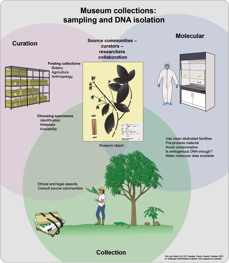
Chapter 2 Infographic: Overview of sampling and obtaining DNA from museum collections. An team effort of communities, curators and researchers (1) Collection of botanical material should have detailed consideration of its ethical and legal aspects and the consultation of source communities in advance, in accordance with CITES, CBD and Nagoya legal and ethical frameworks. (2) Curated botanical samples can be found in different types of museums that include botanic gardens, ethnobotany and anthropological collections. The next step is to find relevant specimens with preferably rich metadata, e.g. species identification, collection place and date. (3) Once the specimens have been identified, they should undergo molecular analyses in clean facilities. Where they will be pre-processed according to their traits, avoiding contamination with other samples, “modern” specimens, and amplicons. Then, it is crucial to identify samples that failed and passed quality controls for endogenous DNA. Finally, the data produced should be linked to their respective vouchers and made available in public repositories like NCBI and BOLD.
Responsible lab use for aDNA
Library-based methods assist with the responsible use of collections, as they preserve the total (non-selective) DNA and ‘immortalise’ it for future use. Immortalisation only has value if the DNA that has been amplified is truly historical/ancient and devoid of contemporary contamination and hence all the aforementioned precautions are necessary when working with aDNA. We recommend that extracts or library builds are precisely annotated with the methods used and are properly archived.
Questions
- Name three legal considerations and their related ethical main issues that should be taken into account for aDNA research using museum material.
- Why is it important to process herbarium samples in a dedicated clean lab?
- Name three benefits of getting curators involved in the early stages of research using collections.
Glossary
aDNA – Ancient DNA, DNA that exhibits biochemical characteristics typical for DNA from old degraded material, i.e., damage and fragmentation, regardless of age.
Artefact – An object made by humans that is of historical or cultural importance, examples include: clothing, ornaments, utensils.
Authentication – Bioinformatic analyses that quantify damage and fragmentation of sequenced DNA to help rule out that DNA is derived from contemporary contamination.
Collection – Repository of curated biological material arranged in a systematic fashion.
Contamination – Introduction of alien tissue or DNA to a specimen or DNA isolate, examples include: microbial colonisation, human epithelium, plant-based foods, etc.
Curator – Custodian of a collection with expert knowledge about specimens, their organisation, and preservation.
Destructive sampling – Permanent removal of a fragment of a specimen of any size that will be irretrievable after biochemical characterization.
DNA damage – Typically conversion of cytosine to uracil in DNA through deamination, which accumulates with time. During sequencing, uracil is replaced with thymine, hence the common synonym, C-to-T substitutions.
Endogenous DNA – Authentic DNA from targeted individuals of a species, in contrast to exogenous DNA from associated microbes and contemporary plant and human DNA contamination.
Fragmentation – Breaks in the DNA backbone, most frequently caused by depurination, leading to shorter DNA fragments with time.
Immortalization – Molecular manipulation of DNA, for example the attachment of DNA adapters, that allows infinite re-amplification of the original DNA from a biological specimen.
Type specimen – Preserved individual plant that has defining features of that taxon that is used for the first taxonomic description of a species. This permanent feature-specimen link is recognized in a publication.
Voucher – Preserved botanical specimen kept in permanent collection and cited by research project. Vouchers will have been expertly identified and are usually annotated with collection time, place, and collector details.
References
- Anderson EN, Pearsall D, Hunn E, Turner N (2011) Ethnobiology. John Wiley & Sons, Inc., Hoboken, NJ, USA. doi: 10.1002/9781118015872
- Austin RM, Sholts SB, Williams L, Kistler L, Hofman CA (2019) Opinion: To curate the molecular past, museums need a carefully considered set of best practices. Proc Natl Acad Sci USA 116, 1471–1474. doi: 10.1073/pnas.1822038116
- Bakker FT, Antonelli A, Clarke JA, Cook JA, Edwards SV, Ericson PGP, Faurby S, Ferrand N, Gelang M, Gillespie RG, Irestedt M, Lundin K, Larsson E, Matos-Maraví P, Müller J, von Proschwitz T, Roderick GK, Schliep A, Wahlberg N, Wiedenhoeft J, Källersjö M (2020) The Global Museum: natural history collections and the future of evolutionary science and public education. PeerJ 8, e8225. doi: 10.7717/peerj.8225
- Bakker FT (2019) Herbarium genomics: plant archival DNA explored, in: Lindqvist, C., Rajora, O.P. (Eds.) Paleogenomics: Genome-Scale Analysis of Ancient DNA, Population Genomics. Springer International Publishing, Cham, pp. 205–224. doi: 10.1007/13836_2018_40
- Bieker VC, Martin MD (2018) Implications and future prospects for evolutionary analyses of DNA in historical herbarium collections. Botany Letters 165, 1–10. doi: 10.1080/23818107.2018.1458651
- Bieker VC, Sánchez Barreiro F, Rasmussen JA, Brunier M, Wales N, Martin MD (2020) Metagenomic analysis of historical herbarium specimens reveals a postmortem microbial community. Mol. Ecol. Resour. 20, 1206–1219. doi: 10.1111/1755-0998.13174
- Briggs AW, Stenzel U, Johnson PLF, Green RE, Kelso J, Prüfer K, Meyer M, Krause J, Ronan MT, Lachmann M, Pääbo S (2007) Patterns of damage in genomic DNA sequences from a Neandertal. Proc Natl Acad Sci USA 104, 14616–14621. doi: 10.1073/pnas.0704665104
- Briggs AW, Stenzel U, Meyer M, Krause J, Kircher M, Pääbo S (2010) Removal of deaminated cytosines and detection of in vivo methylation in ancient DNA. Nucleic Acids Res. 38, e87. doi: 10.1093/nar/gkp1163
- Cappellini E, Gilbert MTP, Geuna F, Fiorentino G, Hall A, Thomas-Oates J, Ashton PD, Ashford DA, Arthur P, Campos PF, Kool J, Willerslev E, Collins MJ (2010) A multidisciplinary study of archaeological grape seeds. Naturwissenschaften 97, 205–217. doi: 10.1007/s00114-009-0629-3
- Carøe C, Gopalakrishnan S, Vinner L, Mak SST, Sinding MHS, Samaniego JA, Wales N, Sicheritz-Pontén T, Gilbert MTP (2017) Single-tube library preparation for degraded DNA. Methods Ecol. Evol. 9, 410–419. doi: 10.1111/2041-210X.12871
- Chomicki G, Renner SS (2015) Watermelon origin solved with molecular phylogenetics including Linnaean material: another example of museomics. New Phytol. 205, 526–532. doi: 10.1111/nph.13163
- Dabney J, Meyer M, Pääbo S (2013) Ancient DNA damage. Cold Spring Harb. Perspect. Biol. 5, a012567. doi: 10.1101/cshperspect.a012567
- Das S, Lowe M (2018) Nature read in black and white: decolonial approaches to interpreting natural history collections. Journal of Natural Science Collections 6, 1–14.
- de Filippo C, Meyer M, Prüfer K (2018) Quantifying and reducing spurious alignments for the analysis of ultra-short ancient DNA sequences. BMC Biol. 16, 121. doi: 10.1186/s12915-018-0581-9
- Durvasula A, Fulgione A, Gutaker RM, Alacakaptan SI, Flood PJ, Neto C, Tsuchimatsu T, Burbano HA, Picó FX, Alonso-Blanco C, Hancock AM (2017) African genomes illuminate the early history and transition to selfing in Arabidopsis thaliana. Proc Natl Acad Sci USA 114, 5213–5218. doi: 10.1073/pnas.1616736114
- Ellis EC, Gauthier N, Klein Goldewijk K, Bliege Bird R, Boivin N, Díaz S, Fuller DQ, Gill JL, Kaplan JO, Kingston N, Locke H, McMichael CNH, Ranco D, Rick TC, Shaw MR, Stephens L, Svenning J-C, Watson JEM (2021) People have shaped most of terrestrial nature for at least 12,000 years. Proc Natl Acad Sci USA 118, e2023483118. doi: 10.1073/pnas.2023483118
- Forrest LL, Hart ML, Hughes M, Wilson HP, Chung K-F, Tseng Y-H, Kidner CA (2019) The limits of Hyb-Seq for herbarium specimens: impact of preservation techniques. Front. Ecol. Evol. 7, 439. doi: 10.3389/fevo.2019.00439
- Freedman J, van Dorp L, Brace S (2018) Destructive sampling natural science collections: An overview for museum professionals and researchers. Journal of Natural Science Collections.
- Fulton TL, Shapiro B (2019) Setting up an ancient DNA laboratory. Methods Mol. Biol. 1963, 1–13. doi: 10.1007/978-1-4939-9176-1_1
- Gewin V (2021) How to include Indigenous researchers and their knowledge. Nature 589, 315–317. doi: 10.1038/d41586-021-00022-1
- Gutaker RM, Burbano HA (2017) Reinforcing plant evolutionary genomics using ancient DNA. Curr. Opin. Plant Biol. 36, 38–45. doi: 10.1016/j.pbi.2017.01.002
- Gutaker RM, Reiter E, Furtwängler A, Schuenemann VJ, Burbano HA (2017) Extraction of ultrashort DNA molecules from herbarium specimens. BioTechniques 62, 76–79. doi: 10.2144/000114517
- Gutaker RM, Weiß CL, Ellis D, Anglin NL, Knapp S, Luis Fernández-Alonso J, Prat S, Burbano HA (2019) The origins and adaptation of European potatoes reconstructed from historical genomes. Nat. Ecol. Evol. 3, 1093–1101. doi: 10.1038/s41559-019-0921-3
- Hodges E, Rooks M, Xuan Z, Bhattacharjee A, Benjamin Gordon D, Brizuela L, Richard McCombie W, Hannon GJ (2009) Hybrid selection of discrete genomic intervals on custom-designed microarrays for massively parallel sequencing. Nat. Protoc. 4, 960–974. doi: 10.1038/nprot.2009.68
- Hofreiter M, Serre D, Poinar HN, Kuch M, Pääbo S (2001) Ancient DNA. Nat. Rev. Genet. 2, 353–359. doi: 10.1038/35072071
- Iob A, Botigué L (2021) Crop archaeogenomics: a powerful resource in need of a well-defined regulation framework. Plants, People, Planet 4, 44–50. doi: 10.1002/ppp3.10233
- Jónsson H, Ginolhac A, Schubert M, Johnson PLF, Orlando L (2013) mapDamage2.0: fast approximate Bayesian estimates of ancient DNA damage parameters. Bioinformatics 29, 1682–1684. doi: 10.1093/bioinformatics/btt193
- Kircher M, Sawyer S, Meyer M (2012) Double indexing overcomes inaccuracies in multiplex sequencing on the Illumina platform. Nucleic Acids Res. 40, e3. doi: 10.1093/nar/gkr771
- Kistler L (2012) Ancient DNA extraction from plants. Methods Mol. Biol. 840, 71–79. doi: 10.1007/978-1-61779-516-9_10
- Latorre SM, Lang PLM, Burbano HA, Gutaker RM (2020) Isolation, library preparation, and bioinformatic analysis of historical and ancient plant DNA. Curr. Protoc. Plant Biol. 5, e20121. doi: 10.1002/cppb.20121
- Maldonado C, Molina CI, Zizka A, Persson C, Taylor CM, Albán J, Chilquillo E, Rønsted N, Antonelli A (2015) Estimating species diversity and distribution in the era of Big Data: to what extent can we trust public databases? Glob. Ecol. Biogeogr. 24, 973–984. doi: 10.1111/geb.12326
- Maricic T, Whitten M, Pääbo S (2010) Multiplexed DNA sequence capture of mitochondrial genomes using PCR products. PLoS ONE 5, e14004. doi: 10.1371/journal.pone.0014004
- Mascher M, Schuenemann VJ, Davidovich U, Marom N, Himmelbach A, Hübner S, Korol A, David M, Reiter E, Riehl S, Schreiber M, Vohr SH, Green RE, Dawson IK, Russell J, Kilian B, Muehlbauer GJ, Waugh R, Fahima T, Krause J, Stein N (2016) Genomic analysis of 6,000-year-old cultivated grain illuminates the domestication history of barley. Nat. Genet. 48, 1089–1093. doi: 10.1038/ng.3611
- McAlvay AC, Armstrong CG, Baker J, Elk LB, Bosco S, Hanazaki N, Joseph L, Martínez-Cruz TE, Nesbitt M, Palmer MA, Priprá de Almeida WC, Anderson J, Asfaw Z, Borokini IT, Cano-Contreras EJ, Hoyte S, Hudson M, Ladio AH, Odonne G, Peter S, Rashford J, Wall J, Wolverton S, Vandebroek I (2021) Ethnobiology phase VI: decolonizing institutions, projects, and scholarship. J. Ethnobiol. 41, 170–191. doi: 10.2993/0278-0771-41.2.170
- McManis CR, Pelletier JS (2014) Legal aspects of biocultural collections, in: Salick, J., Konchar, K., Nesbitt, M. (Eds.) Presented at the Curating biocultural collections: a handbook, Royal Botanic Gardens, Kew, Kew, pp. 229–243.
- Meyer M, Kircher M, Gansauge M-T, Li H, Racimo F, Mallick S, Schraiber JG, Jay F, Prüfer K, de Filippo C, Sudmant PH, Alkan C, Fu Q, Do R, Rohland N, Tandon A, Siebauer M, Green RE, Bryc K, Briggs AW, Pääbo S (2012) A high-coverage genome sequence from an archaic Denisovan individual. Science 338, 222–226. doi: 10.1126/science.1224344
- Meyer M, Kircher M (2010) Illumina sequencing library preparation for highly multiplexed target capture and sequencing. Cold Spring Harb. Protoc. 2010, pdb.prot5448. doi: 10.1101/pdb.prot5448
- Nesbitt M, Colledge S, Murray MA (2003) Organisation and management of seed reference collections. Environmental Archaeology 8, 77–84. doi: 10.1179/env.2003.8.1.77
- Nistelberger HM, Smith O, Wales N, Star B, Boessenkool S (2016) The efficacy of high-throughput sequencing and target enrichment on charred archaeobotanical remains. Sci. Rep. 6, 37347. doi: 10.1038/srep37347
- Overballe-Petersen S, Orlando L, Willerslev E (2012) Next-generation sequencing offers new insights into DNA degradation. Trends Biotechnol. 30, 364–368. doi: 10.1016/j.tibtech.2012.03.007
- Pääbo S, Poinar H, Serre D, Jaenicke-Despres V, Hebler J, Rohland N, Kuch M, Krause J, Vigilant L, Hofreiter M (2004) Genetic analyses from ancient DNA. Annu. Rev. Genet. 38, 645–679. doi: 10.1146/annurev.genet.37.110801.143214
- Pálsdóttir AH, Bläuer A, Rannamäe E, Boessenkool S, Hallsson JH (2019) Not a limitless resource: ethics and guidelines for destructive sampling of archaeofaunal remains. R. Soc. Open Sci. 6, 191059. doi: 10.1098/rsos.191059
- Peltzer A, Jäger G, Herbig A, Seitz A, Kniep C, Krause J, Nieselt K (2016) EAGER: efficient ancient genome reconstruction. Genome Biol. 17, 60. doi: 10.1186/s13059-016-0918-z
- Pont C, Wagner S, Kremer A, Orlando L, Plomion C, Salse J (2019) Paleogenomics: reconstruction of plant evolutionary trajectories from modern and ancient DNA. Genome Biol. 20, 29. doi: 10.1186/s13059-019-1627-1
- Prüfer K, Stenzel U, Hofreiter M, Pääbo S, Kelso J, Green RE (2010) Computational challenges in the analysis of ancient DNA. Genome Biol. 11, R47. doi: 10.1186/gb-2010-11-5-r47
- Pungetti G, Oviedo G, Hooke D (2012) Sacred species and sites: advances in biocultural conservation. Cambridge University Press, Cambridge. doi: 10.1017/CBO9781139030717
- Ratsch A, Steadman KJ, Bogossian F (2010) The pituri story: a review of the historical literature surrounding traditional Australian Aboriginal use of nicotine in Central Australia. J. Ethnobiol. Ethnomed. 6, 26. doi: 10.1186/1746-4269-6-26
- Rivier L, Lindgren J-E (1972) “Ayahuasca,” the South American hallucinogenic drink: an ethnobotanical and chemical investigation. Econ. Bot. 26, 101–129. doi: 10.1007/BF02860772
- Salick J, Konchar K, Nesbitt M (2014) Curating Biocultural Collections: A Handbook. Royal Botanic Gardens, Kew, Kew.
- Schindel DE, Cook JA (2018) The next generation of natural history collections. PLoS Biol. 16, e2006125. doi: 10.1371/journal.pbio.2006125
- Schrader C, Schielke A, Ellerbroek L, Johne R (2012) PCR inhibitors - occurrence, properties and removal. J. Appl. Microbiol. 113, 1014–1026. doi: 10.1111/j.1365-2672.2012.05384.x
- Schubert M, Ermini L, Der Sarkissian C, Jónsson H, Ginolhac A, Schaefer R, Martin MD, Fernández R, Kircher M, McCue M, Willerslev E, Orlando L (2014) Characterization of ancient and modern genomes by SNP detection and phylogenomic and metagenomic analysis using PALEOMIX. Nat. Protoc. 9, 1056–1082. doi: 10.1038/nprot.2014.063
- Scott MF, Botigué LR, Brace S, Stevens CJ, Mullin VE, Stevenson A, Thomas MG, Fuller DQ, Mott R (2019) A 3,000-year-old Egyptian emmer wheat genome reveals dispersal and domestication history. Nat. Plants 5, 1120–1128. doi: 10.1038/s41477-019-0534-5
- Sherman B, Henry RJ (2020) The Nagoya Protocol and historical collections of plants. Nat. Plants 6, 430–432. doi: 10.1038/s41477-020-0657-8
- Staats M, Erkens RHJ, van de Vossenberg B, Wieringa JJ, Kraaijeveld K, Stielow B, Geml J, Richardson JE, Bakker FT (2013) Genomic treasure troves: complete genome sequencing of herbarium and insect museum specimens. PLoS ONE 8, e69189. doi: 10.1371/journal.pone.0069189
- Swarts K, Gutaker RM, Benz B, Blake M, Bukowski R, Holland J, Kruse-Peeples M, Lepak N, Prim L, Romay MC, Ross-Ibarra J, Sanchez-Gonzalez J de J, Schmidt C, Schuenemann VJ, Krause J, Matson RG, Weigel D, Buckler ES, Burbano HA (2017) Genomic estimation of complex traits reveals ancient maize adaptation to temperate North America. Science 357, 512–515. doi: 10.1126/science.aam9425
- Van de Paer C, Hong-Wa C, Jeziorski C, Besnard G (2016) Mitogenomics of Hesperelaea, an extinct genus of Oleaceae. Gene 594, 197–202. doi: 10.1016/j.gene.2016.09.007
- Wagner S, Lagane F, Seguin-Orlando A, Schubert M, Leroy T, Guichoux E, Chancerel E, Bech-Hebelstrup I, Bernard V, Billard C, Billaud Y, Bolliger M, Croutsch C, Čufar K, Eynaud F, Heussner KU, Köninger J, Langenegger F, Leroy F, Lima C, Orlando L (2018) High-Throughput DNA sequencing of ancient wood. Mol. Ecol. 27, 1138–1154. doi: 10.1111/mec.14514
- Wales N, Andersen K, Cappellini E, Avila-Arcos MC, Gilbert MTP (2014) Optimization of DNA recovery and amplification from non-carbonized archaeobotanical remains. PLoS ONE 9, e86827. doi: 10.1371/journal.pone.0086827
- Wales N, Kistler L (2019) Extraction of ancient DNA from plant remains. Methods Mol. Biol. 1963, 45–55. doi: 10.1007/978-1-4939-9176-1_6
- Weiß CL, Schuenemann VJ, Devos J, Shirsekar G, Reiter E, Gould BA, Stinchcombe JR, Krause J, Burbano HA (2016) Temporal patterns of damage and decay kinetics of DNA retrieved from plant herbarium specimens. R. Soc. Open Sci. 3, 160239. doi: 10.1098/rsos.160239
Answers
- Legal: CITES (restriction in international trade of endangered species), Nagoya Protocol (ownership and other significance to indigenous peoples), and Drug Act (controlled substances).
- The decay of DNA from historical plant material makes it very susceptible to contamination with exogenous modern DNA.
- Curators can contribute (1) high-quality metadata such as collection dates and provenance, (2) knowledge of collections in-house and elsewhere, (3) knowledge of source communities and ethical and legal issues, (4) advice on choice of specimens most suitable for sampling.
Chapter 3 DNA from water
Introduction
The first studies conducted on DNA obtained from water samples were published in the 1990s. Cloning techniques were commonly used to investigate novel genes and functions of environmental communities at that time. Stein et al. (
Conventionally, biomonitoring of freshwater and marine environments is based on direct observation of indicator taxa to compute biotic metrics/indices. This can be time and labour intensive (
The main advantage of water is the ease of sample collection compared to other aquatic sample types such as sediments or biofilms, as these substrates usually require more sophisticated tools and longer sampling times (
Detecting DNA in water samples obtained from aquatic environments can be challenging because it is usually present at low concentrations with an uneven spatial distribution (
Detection of DNA from aquatic environments
Natural processes influencing the composition and quantity of detectable DNA in a water sample can be categorised into 1) shedding of biological material from source organisms, 2) degradation, 3) transport across the water column, and 4) retention and resuspension (
Shedding
Senescence in aquatic plants releases free cells into the water column that will eventually break down into organic compounds, including DNA. However, degradation in many cells begins via apoptosis before shedding. Apoptosis involves the shrinkage of the cell and its nucleus in a programmed way, in contrast to necrosis, which is uncontrolled cell death due to loss of osmotic control typically by swelling and bursting (
DNA degradation
DNA is a highly stable molecule at neutral pH and moderate temperatures. However, there are several abiotic factors that directly and indirectly influence its stability in aquatic environments (
Transportation, retention, and resuspension
Hydrological characteristics of the water body are also critical to consider when inferring species presence and distribution. DNA can bind to particles of varying size in aquatic environments (less than 0.2 µm to greater than 180 µm) and this particle association is one of many parameters that affect DNA transport and diffusion (
Considering the higher dilution and the effects of currents and waves in marine waters, DNA is generally less concentrated and more quickly dispersed compared to freshwater ecosystems (
In rivers and streaming waters, the probability of DNA detection is strongly correlated with downstream transportation rates. Retention, rather than degradation, appears to be a more important factor that limits the transport of DNA in streaming waters (
Targeted approaches and community analyses using plant DNA from water
Conventional sampling techniques often require a lot of time and effort for detecting indicator, rare, or invasive species. Keeping the target organism alive or intact might also be an important consideration in such cases. Detection of species via nucleic acids collected from environmental samples (eDNA/eRNA) is a relatively new approach that emerged in the last five years (Anglès d’Auriac et al. 2019). These methods offer a non-destructive and efficient complementary approach for the detection of aquatic organisms. They rely on reference sequences and the amount of available data varies among taxonomic groups and countries (Chapter 10 DNA barcoding and Chapter 11 Amplicon metabarcoding). For example, aquatic vascular plants used in biomonitoring are well represented in public databases (BOLD, GenBank), while this is hard to achieve for diatoms due to large proportions of undescribed species and the problems with cultivation of monoclonal cultures (
Although DNA from plant communities have been detected from environmental samples as parts of larger surveys (e.g., within coral reefs), biodiversity studies targeting a large number of plant species are still rare, possibly owing to issues with universal amplification and discriminatory power of single or multiple gene surveys in plants (
An important application for DNA-based methods is the quantification of species abundance and biomass since there are several environmental applications that rely on this information. Depending on the specific aim of the study, this information can be obtained at varying degrees of efficiency and reliability. Approaches employing species-specific methods are more suitable for abundance or biomass estimations (e.g., qPCR, ddPCR). However, they require a priori knowledge of the target group and are limited to already described species. On the other hand, high-throughput approaches can identify species that are rare or have low biomass (e.g., metabarcoding, metagenomics), but they suffer from biases introduced by downstream steps such as PCR amplification, sequencing (Chapter 9 Sequencing platforms and data types), availability of reference sequences, and even the bioinformatics analyses (Chapter 18 Sequence to species) (
Although molecular methods for species detection have been used as a tool for biodiversity management for more than a decade, only 2% of the available studies have focused on plants (
Experimental design
Recent studies that detect plant species in aquatic ecosystems via eDNA are mainly about methodological adjustments (
Sampling strategies: water collection, filtering, and transportation
There are three main steps in a field study for the collection of aqueous eDNA: water collection, transportation, and filtering. In designing sampling strategies for species identification from water samples, there are many factors to consider. These include, but are not limited to, the field conditions, the distance between sampling point and laboratory, the amount of water that is required, and the morphology and life cycle of the target organism (
After the selection of the sampling location, the next step is to decide on the transportation strategy. Water samples can either be directly transported to the laboratory or filtered in the field. If direct transportation is the chosen method, the samples are usually collected with sterilised glass or plastic bottles or disposable plastic tubes. After that, DNA in the water samples can be captured by filtration or ethanol precipitation in the laboratory. This method both reduces the effort and time spent in the field and researchers can perform additional analyses on water samples or store subsamples for further processing (
Precipitation using ethanol or isopropanol can be used for capturing DNA after water collection, but filtration is the more widely used method (
Pore sizes of filters used in eDNA studies range from 0.22 µm to 60 µm (
The type of filter is one of the most important decisions to be made when designing the sampling strategy. Filters can be classified as open or encapsulated/cartridge filters (
Contamination of samples and the degradation of DNA are two critical processes that should be avoided as much as possible from water collection in the field to DNA isolation in the lab (
DNA extraction
Choosing the correct DNA extraction protocol can be crucial in ensuring that the effect of PCR inhibitors in water samples will be minimised. The chemical and physical characteristics of samples can vary considerably, and therefore the quantity and purity of isolated DNA also vary (

Chapter 3 Infographic: Summary of steps from field collection of water samples to DNA extraction in the laboratory. (1) Open or closed (encapsulated/cartridge) filters can be used for filtering water samples on-site. Large filters (e.g., plankton net with 60 μm pore size) are preferred for filtering larger volumes of water, while small pore size filters can usually process a few litres. Closed filters offer the advantage of preventing contamination, therefore they are more commonly used for on-site filtration. (2) Degradation is another important issue that should be prevented until DNA extraction. Water or filter samples can either be preserved in a chemical buffer or transported in cold and dark conditions to the laboratory for further processing. (3) Plant DNA in water samples can be captured by filtration or precipitation. When using filtration, samples are usually incubated in a lysis solution to extract DNA, while in precipitation samples are mixed with ethanol and DNA is collected in the pellet. Commercial DNA isolation kits specifically designed for environmental sample types are commonly used with some small modifications.
Conclusion and prospects
DNA isolated from water samples can be used for several downstream applications based on the specific aim of the study or survey. Currently, qPCR methods are the most commonly used method for detecting specific target taxa in water samples, while metabarcoding is used for community analyses (Chapter 11 Metabarcoding). The studies comparing the efficiency of these DNA methods with more conventional methods show varying results. For some species or taxa, DNA-based detection methods appear to outperform more conventional methods (
Questions
- Are water samples best collected at a single point representative of the habitat diversity as a whole? Motivate your answer.
- Describe three biotic and three abiotic factors that can affect DNA detection rates in aquatic environments. Explain in a few sentences how these factors can result in the detection of false positives and false negatives in streaming waters.
- List five factors that should be taken into account while designing a sampling strategy for detection of DNA from water samples.
Glossary
Apoptosis – Controlled cell death which involves cell shrinkage, nuclear fragmentation, chromatin condensation, and chromosomal DNA fragmentation.
Biofilm – A consortium of microorganisms where cells stick to each other and often also to a surface.
Dimictic lake – A body of freshwater whose difference in temperature between surface and bottom layers becomes negligible twice per year.
Extracellular nucleases – Enzymes that can work outside of the cell and are capable of cleaving the phosphodiester bonds between nucleotides of nucleic acids.
Mesocosm – Any outdoor experimental system that simulates the natural environment under controlled conditions.
Necrosis – Uncontrolled cell death due to the loss of osmotic control typically by swelling and bursting.
PCR inhibitors – Any factor which prevents the amplification of nucleic acids through the polymerase chain reaction.
Primer – A short single stranded nucleic acid sequence used by all living organisms in the initiation of DNA synthesis.
qPCR (Quantitative PCR) – An extension of the PCR technique which allows estimation of the initial quantity of nucleic acids in a biological sample.
Senescence – The gradual deterioration of functional characteristics with ageing (can be used both for organismal or cellular ageing).
Thermal stratification – The phenomenon in which lakes develop two discrete layers of water of different temperatures; warm on top (epilimnion) and cold below (hypolimnion).
Vector (i.e., cloning vectors) – A small piece of DNA that can be stably maintained in an organism that a foreign DNA fragment can be inserted into for cloning purposes.
References
- Alsos IG, Lammers Y, Yoccoz NG, Jørgensen T, Sjögren P, Gielly L, Edwards ME (2018) Plant DNA metabarcoding of lake sediments: How does it represent the contemporary vegetation. PLoS ONE 13, e0195403. doi: 10.1371/journal.pone.0195403
- Anglès d’Auriac MB, Strand DA, Mjelde M, Demars BOL, Thaulow J (2019) Detection of an invasive aquatic plant in natural water bodies using environmental DNA. PLoS ONE 14, e0219700. doi: 10.1371/journal.pone.0219700
- Apothéloz-Perret-Gentil L, Bouchez A, Cordier T, Cordonier A, Guéguen J, Rimet F, Vasselon V, Pawlowski J (2021) Monitoring the ecological status of rivers with diatom eDNA metabarcoding: A comparison of taxonomic markers and analytical approaches for the inference of a molecular diatom index. Mol. Ecol. 30, 2959–2968. doi: 10.1111/mec.15646
- Barnes MA, Turner CR, Jerde CL, Renshaw MA, Chadderton WL, Lodge DM (2014) Environmental conditions influence eDNA persistence in aquatic systems. Environ. Sci. Technol. 48, 1819–1827. doi: 10.1021/es404734p
- Beng KC, Corlett RT (2020) Applications of environmental DNA (eDNA) in ecology and conservation: opportunities, challenges and prospects. Biodivers. Conserv. 29, 2089–2121. doi: 10.1007/s10531-020-01980-0
- Bista I, Carvalho GR, Walsh K, Seymour M, Hajibabaei M, Lallias D, Christmas M, Creer S (2017) Annual time-series analysis of aqueous eDNA reveals ecologically relevant dynamics of lake ecosystem biodiversity. Nat. Commun. 8, 14087. doi: 10.1038/ncomms14087
- Bruce K, Blackman R, Bourlat SJ, Hellstrom AM, Bakker J, Bista I, Bohmann K, Bouchez A, Brys R, Clark K, Elbrecht V, Fazi S, Fonseca V, Hänfling B, Leese F, Mächler E, Mahon AR, Meissner K, Panksep K, Pawlowski J, Deiner K (2021) A practical guide to DNA-based methods for biodiversity assessment. Pensoft Publishers. doi: 10.3897/ab.e68634
- Carim KJ, McKelvey KS, Young MK, Wilcox TM, Schwartz MK (2016) A protocol for collecting environmental DNA samples from streams. U.S. Department of Agriculture, Forest Service, Rocky Mountain Research Station, Ft. Collins, CO. doi: 10.2737/RMRS-GTR-355
- Carraro L, Mächler E, Wüthrich R, Altermatt F (2020) Environmental DNA allows upscaling spatial patterns of biodiversity in freshwater ecosystems. Nat. Commun. 11, 3585. doi: 10.1038/s41467-020-17337-8
- Carraro L, Stauffer JB, Altermatt F (2021) How to design optimal eDNA sampling strategies for biomonitoring in river networks. Environmental DNA 3, 157–172. doi: 10.1002/edn3.137
- Coghlan SA, Shafer ABA, Freeland JR (2020) Development of an environmental DNA metabarcoding assay for aquatic vascular plant communities. Environmental DNA. doi: 10.1002/edn3.120
- Collins RA, Wangensteen OS, O’Gorman EJ, Mariani S, Sims DW, Genner MJ (2018) Persistence of environmental DNA in marine systems. Commun. Biol. 1, 185. doi: 10.1038/s42003-018-0192-6
- D’Alessandro S, Mariani S (2021) Sifting environmental DNA metabarcoding data sets for rapid reconstruction of marine food webs. Fish Fish. doi: 10.1111/faf.12553
- Deiner K, Bik HM, Mächler E, Seymour M, Lacoursière-Roussel A, Altermatt F, Creer S, Bista I, Lodge DM, de Vere N, Pfrender ME, Bernatchez L (2017) Environmental DNA metabarcoding: Transforming how we survey animal and plant communities. Mol. Ecol. 26, 5872–5895. doi: 10.1111/mec.14350
- Deiner K, Fronhofer EA, Mächler E, Walser J-C, Altermatt F (2016) Environmental DNA reveals that rivers are conveyer belts of biodiversity information. Nat. Commun. 7, 12544. doi: 10.1038/ncomms12544
- Dejean T, Valentini A, Duparc A, Pellier-Cuit S, Pompanon F, Taberlet P, Miaud C (2011) Persistence of environmental DNA in freshwater ecosystems. PLoS ONE 6, e23398. doi: 10.1371/journal.pone.0023398
- de Souza LS, Godwin JC, Renshaw MA, Larson E (2016) Environmental DNA (edna) detection probability is influenced by seasonal activity of organisms. PLoS ONE 11, e0165273. doi: 10.1371/journal.pone.0165273
- DiBattista JD, Reimer JD, Stat M, Masucci GD, Biondi P, De Brauwer M, Bunce M (2019) Digging for DNA at depth: rapid universal metabarcoding surveys (RUMS) as a tool to detect coral reef biodiversity across a depth gradient. PeerJ 7, e6379. doi: 10.7717/peerj.6379
- Eichmiller JJ, Best SE, Sorensen PW (2016) Effects of temperature and trophic state on degradation of environmental DNA in lake water. Environ. Sci. Technol. 50, 1859–1867. doi: 10.1021/acs.est.5B010305672
- Ficetola GF, Miaud C, Pompanon F, Taberlet P (2008) Species detection using environmental DNA from water samples. Biol. Lett. 4, 423–425. doi: 10.1098/rsbl.2008.0118
- Foote AD, Thomsen PF, Sveegaard S, Wahlberg M, Kielgast J, Kyhn LA, Salling AB, Galatius A, Orlando L, Gilbert MTP (2012) Investigating the potential use of environmental DNA (eDNA) for genetic monitoring of marine mammals. PLoS ONE 7, e41781. doi: 10.1371/journal.pone.0041781
- Foran DR (2006) Relative degradation of nuclear and mitochondrial DNA: an experimental approach. J. Forensic Sci. 51, 766–770. doi: 10.1111/j.1556-4029.2006.00176.x
- Fraser CI, Connell L, Lee CK, Cary SC (2017) Evidence of plant and animal communities at exposed and subglacial (cave) geothermal sites in Antarctica. Polar Biol. 41, 1–5. doi: 10.1007/s00300-017-2198-9
- Fujiwara A, Matsuhashi S, Doi H, Yamamoto S, Minamoto T (2016) Use of environmental DNA to survey the distribution of an invasive submerged plant in ponds. Freshwater Science 35, 748–754. doi: 10.1086/685882
- Fukaya K, Murakami H, Yoon S, Minami K, Osada Y, Yamamoto S, Masuda R, Kasai A, Miyashita K, Minamoto T, Kondoh M (2020) Estimating fish population abundance by integrating quantitative data on environmental DNA and hydrodynamic modelling. Mol. Ecol. doi: 10.1111/mec.15530
- Gantz CA, Renshaw MA, Erickson D, Lodge DM, Egan SP (2018) Environmental DNA detection of aquatic invasive plants in lab mesocosm and natural field conditions. Biol. Invasions 20, 1–18. doi: 10.1007/s10530-018-1718-z
- Goldberg CS, Turner CR, Deiner K, Klymus KE, Thomsen PF, Murphy MA, Spear SF, McKee A, Oyler-McCance SJ, Cornman RS, Laramie MB, Mahon AR, Lance RF, Pilliod DS, Strickler KM, Waits LP, Fremier AK, Takahara T, Herder JE, Taberlet P (2016) Critical considerations for the application of environmental DNA methods to detect aquatic species. Methods Ecol. Evol. doi: 10.1111/2041-210X.12595
- Hajibabaei M, Shokralla S, Zhou X, Singer GAC, Baird DJ (2011) Environmental barcoding: a next-generation sequencing approach for biomonitoring applications using river benthos. PLoS ONE 6, e17497. doi: 10.1371/journal.pone.0017497
- Harper LR, Buxton AS, Rees HC, Bruce K, Brys R, Halfmaerten D, Read DS, Watson HV, Sayer CD, Jones EP, Priestley V, Mächler E, Múrria C, Garcés-Pastor S, Medupin C, Burgess K, Benson G, Boonham N, Griffiths RA, Lawson Handley L, Hänfling B (2019) Prospects and challenges of environmental DNA (eDNA) monitoring in freshwater ponds. Hydrobiologia 826, 25–41. doi: 10.1007/s10750-018-3750-5
- Harrison JB, Sunday JM, Rogers SM (2019) Predicting the fate of eDNA in the environment and implications for studying biodiversity. Proc. Biol. Sci. 286, 20191409. doi: 10.1098/rspb.2019.1409
- Hinlo R, Gleeson D, Lintermans M, Furlan E (2017) Methods to maximise recovery of environmental DNA from water samples. PLoS ONE 12, e0179251. doi: 10.1371/journal.pone.0179251
- Hofreiter M, Serre D, Poinar HN, Kuch M, Pääbo S (2001) Ancient DNA. Nat. Rev. Genet. 2, 353–359. doi: 10.1038/35072071
- Hotchkiss RS, Strasser A, McDunn JE, Swanson PE (2009) Cell death. N. Engl. J. Med. 361, 1570–1583. doi: 10.1056/NEJMra0901217
- Hunter ME, Ferrante JA, Meigs-Friend G, Ulmer A (2019) Improving eDNA yield and inhibitor reduction through increased water volumes and multi-filter isolation techniques. Sci. Rep. 9, 5259. doi: 10.1038/s41598-019-40977-w
- Kelly RP, Gallego R, Jacobs-Palmer E (2018) The effect of tides on nearshore environmental DNA. PeerJ 6, e4521. doi: 10.7717/peerj.4521
- Kuehne LM, Ostberg CO, Chase DM, Duda JJ, Olden JD (2020) Use of environmental DNA to detect the invasive aquatic plants Myriophyllum spicatum and Egeria densa in lakes. Freshwater Science 39, 521–533. doi: 10.1086/710106
- Laramie MB, Pilliod DS, Goldberg CS, Strickler KM (2015) Environmental DNA sampling protocol - filtering water to capture DNA from aquatic organisms. Techniques and Methods.
- Leech DM, Snyder MT, Wetzel RG (2009) Natural organic matter and sunlight accelerate the degradation of 17ss-estradiol in water. Sci. Total Environ. 407, 2087–2092. doi: 10.1016/j.scitotenv.2008.11.018
- Mächler E, Salyani A, Walser J-C, Larsen A, Schaefli B, Altermatt F, Ceperley N (2021) Environmental DNA simultaneously informs hydrological and biodiversity characterization of an Alpine catchment. Hydrol. Earth Syst. Sci. 25, 735–753. doi: 10.5194/hess-25-735-2021
- Matsuhashi S, Doi H, Fujiwara A, Watanabe S, Minamoto T (2016) Evaluation of the environmental DNA method for estimating distribution and biomass of submerged aquatic plants. PLoS ONE 11, e0156217. doi: 10.1371/journal.pone.0156217
- Matsuhashi S, Minamoto T, Doi H (2019) Seasonal change in environmental DNA concentration of a submerged aquatic plant species. Freshwater Science 38, 654–660. doi: 10.1086/704996
- Minamoto T, Naka T, Moji K, Maruyama A (2016) Techniques for the practical collection of environmental DNA: filter selection, preservation, and extraction. Limnology 17, 23–32. doi: 10.1007/s10201-015-0457-4
- Miyazono S, Kodama T, Akamatsu Y, Nakao R, Saito M (2020) Application of environmental DNA methods for the detection and abundance estimation of invasive aquatic plant Egeria densa in lotic habitats. Limnology. doi: 10.1007/s10201-020-00636-w
- Muha TP, Skukan R, Borrell YJ, Rico JM, Garcia de Leaniz C, Garcia-Vazquez E, Consuegra S (2019) Contrasting seasonal and spatial distribution of native and invasive Codium seaweed revealed by targeting species-specific eDNA. Ecol. Evol. 9, 8567–8579. doi: 10.1002/ece3.5379
- Nowak P, Wiebe C, Karez R, Schubert H (2021) Applications of environmental DNA methods for charophyte biodiversity. ACA 4. doi: 10.3897/aca.4.e64944
- Noyer C, Abot A, Trouilh L, Leberre VA, Dreanno C (2015) Phytochip: development of a DNA-microarray for rapid and accurate identification of Pseudo-nitzschia spp and other harmful algal species. J. Microbiol. Methods 112, 55–66. doi: 10.1016/j.mimet.2015.03.002
- Okabe S, Shimazu Y (2007) Persistence of host-specific Bacteroides-Prevotella 16S rRNA genetic markers in environmental waters: effects of temperature and salinity. Appl. Microbiol. Biotechnol. 76, 935–944. doi: 10.1007/s00253-007-1048-z
- Pawlowski J, Kelly-Quinn M, Altermatt F, Apothéloz-Perret-Gentil L, Beja P, Boggero A, Borja A, Bouchez A, Cordier T, Domaizon I, Feio MJ, Filipe AF, Fornaroli R, Graf W, Herder J, van der Hoorn B, Iwan Jones J, Sagova-Mareckova M, Moritz C, Barquín J, Kahlert M (2018) The future of biotic indices in the ecogenomic era: Integrating (e)DNA metabarcoding in biological assessment of aquatic ecosystems. Sci. Total Environ. 637–638, 1295–1310. doi: 10.1016/j.scitotenv.2018.05.002
- Pilliod DS, Goldberg CS, Arkle RS, Waits LP (2014) Factors influencing detection of eDNA from a stream-dwelling amphibian. Mol. Ecol. Resour. 14, 109–116. doi: 10.1111/1755-0998.12159
- Pont D, Rocle M, Valentini A, Civade R, Jean P, Maire A, Roset N, Schabuss M, Zornig H, Dejean T (2018) Environmental DNA reveals quantitative patterns of fish biodiversity in large rivers despite its downstream transportation. Sci. Rep. 8, 10361. doi: 10.1038/s41598-018-28424-8
- Poté J, Ackermann R, Wildi W (2009) Plant leaf mass loss and DNA release in freshwater sediments. Ecotoxicol. Environ. Saf. 72, 1378–1383. doi: 10.1016/j.ecoenv.2009.04.010
- Reape TJ, Molony EM, McCabe PF (2008) Programmed cell death in plants: distinguishing between different modes. J. Exp. Bot. 59, 435–444. doi: 10.1093/jxb/erm258
- Rose JP, Wademan C, Weir S, Wood JS, Todd BD (2019) Traditional trapping methods outperform eDNA sampling for introduced semi-aquatic snakes. PLoS ONE 14, e0219244. doi: 10.1371/journal.pone.0219244
- Schabacker JC, Amish SJ, Ellis BK, Gardner B, Miller DL, Rutledge EA, Sepulveda AJ, Luikart G (2020) Increased eDNA detection sensitivity using a novel high-volume water sampling method. Environmental DNA 2, 244–251. doi: 10.1002/edn3.63
- Schroeder GK, Wolfenden R (2007) Rates of spontaneous disintegration of DNA and the rate enhancements produced by DNA glycosylases and deaminases. Biochemistry 46, 13638–13647. doi: 10.1021/bi701480f
- Scriver M, Marinich A, Wilson C, Freeland J (2015) Development of species-specific environmental DNA (eDNA) markers for invasive aquatic plants. Aquatic Botany 122, 27–31. doi: 10.1016/j.aquabot.2015.01.003
- Sepulveda AJ, Schabacker J, Smith S, Al-Chokhachy R, Luikart G, Amish SJ (2019) Improved detection of rare, endangered and invasive trout in using a new large-volume sampling method for eDNA capture. Environmental DNA 1, 227–237. doi: 10.1002/edn3.23
- Shackleton ME, Rees GN, Watson G, Campbell C, Nielsen D (2019) Environmental DNA reveals landscape mosaic of wetland plant communities. Glob. Ecol. Conserv. 19, e00689. doi: 10.1016/j.gecco.2019.e00689
- Shogren AJ, Tank JL, Andruszkiewicz EA, Olds B, Jerde C, Bolster D (2016) Modelling the transport of environmental DNA through a porous substrate using continuous flow-through column experiments. J. R. Soc. Interface 13. doi: 10.1098/rsif.2016.0290
- Shogren AJ, Tank JL, Egan SP, August O, Rosi EJ, Hanrahan BR, Renshaw MA, Gantz CA, Bolster D (2018) Water flow and biofilm cover influence environmental DNA detection in recirculating streams. Environ. Sci. Technol. 52, 8530–8537. doi: 10.1021/acs.est.8B010301822
- Singer GAC, Fahner NA, Barnes JG, McCarthy A, Hajibabaei M (2019) Comprehensive biodiversity analysis via ultra-deep patterned flow cell technology: a case study of eDNA metabarcoding seawater. Sci. Rep. 9, 5991. doi: 10.1038/s41598-019-42455-9
- Spens J, Evans AR, Halfmaerten D, Knudsen SW, Sengupta ME, Mak SST, Sigsgaard EE, Hellström M (2017) Comparison of capture and storage methods for aqueous macrobial eDNA using an optimized extraction protocol: advantage of enclosed filter. Methods Ecol. Evol. 8, 635–645. doi: 10.1111/2041-210X.12683
- Stein JL, Marsh TL, Wu KY, Shizuya H, DeLong EF (1996) Characterization of uncultivated prokaryotes: isolation and analysis of a 40-kilobase-pair genome fragment from a planktonic marine archaeon. J. Bacteriol. 178, 591–599. doi: 10.1128/jb.178.3.591-599.1996
- Strickler KM, Fremier AK, Goldberg CS (2015) Quantifying effects of UV-B, temperature, and pH on eDNA degradation in aquatic microcosms. Biological Conservation 183, 85–92. doi: 10.1016/j.biocon.2014.11.038
- Thomas AC, Nguyen PL, Howard J, Goldberg CS (2019) A self-preserving, partially biodegradable eDNA filter. Methods Ecol. Evol. 10, 1136–1141. doi: 10.1111/2041-210X.13212
- Thomsen PF, Kielgast J, Iversen LL, Wiuf C, Rasmussen M, Gilbert MTP, Orlando L, Willerslev E (2012) Monitoring endangered freshwater biodiversity using environmental DNA. Mol. Ecol. 21, 2565–2573. doi: 10.1111/j.1365-294X.2011.05418.x
- Tingley R, Greenlees M, Oertel S, van Rooyen AR, Weeks AR (2018) Environmental DNA sampling as a surveillance tool for cane toad Rhinella marina introductions on offshore islands. Biol. Invasions 1–6. doi: 10.1007/s10530-018-1810-4
- Toné S, Sugimoto K, Tanda K, Suda T, Uehira K, Kanouchi H, Samejima K, Minatogawa Y, Earnshaw WC (2007) Three distinct stages of apoptotic nuclear condensation revealed by time-lapse imaging, biochemical and electron microscopy analysis of cell-free apoptosis. Exp. Cell Res. 313, 3635–3644. doi: 10.1016/j.yexcr.2007.06.018
- Tsuji S, Takahara T, Doi H, Shibata N, Yamanaka H (2019) The detection of aquatic macroorganisms using environmental DNA analysis—A review of methods for collection, extraction, and detection. Environmental DNA 1, 99–108. doi: 10.1002/edn3.21
- Tsuji S, Ushio M, Sakurai S, Minamoto T, Yamanaka H (2017) Water temperature-dependent degradation of environmental DNA and its relation to bacterial abundance. PLoS ONE 12, e0176608. doi: 10.1371/journal.pone.0176608
- Turner CR, Barnes MA, Xu CCY, Jones SE, Jerde CL, Lodge DM (2014) Particle size distribution and optimal capture of aqueous macrobial eDNA. Methods Ecol. Evol. 5, 676–684. doi: 10.1111/2041-210X.12206
- Turner CR, Uy KL, Everhart RC (2015) Fish environmental DNA is more concentrated in aquatic sediments than surface water. Biological Conservation 183, 93–102. doi: 10.1016/j.biocon.2014.11.017
- Vanyushin BF, Bakeeva LE, Zamyatnina VA, Aleksandrushkina NI (2004) Apoptosis in plants: specific features of plant apoptotic cells and effect of various factors and agents. Int. Rev. Cytol. 233, 135–179. doi: 10.1016/S0074-7696(04)33004-4
- Venter JC, Remington K, Heidelberg JF, Halpern AL, Rusch D, Eisen JA, Wu D, Paulsen I, Nelson KE, Nelson W, Fouts DE, Levy S, Knap AH, Lomas MW, Nealson K, White O, Peterson J, Hoffman J, Parsons R, Baden-Tillson H, Smith HO (2004) Environmental genome shotgun sequencing of the Sargasso Sea. Science 304, 66–74. doi: 10.1126/science.1093857
- Weigand H, Beermann AJ, Čiampor F, Costa FO, Csabai Z, Duarte S, Geiger MF, Grabowski M, Rimet F, Rulik B, Strand M, Szucsich N, Weigand AM, Willassen E, Wyler SA, Bouchez A, Borja A, Čiamporová-Zaťovičová Z, Ferreira S, Dijkstra K-DB, Ekrem T (2019) DNA barcode reference libraries for the monitoring of aquatic biota in Europe: Gap-analysis and recommendations for future work. Sci. Total Environ. 678, 499–524. doi: 10.1016/j.scitotenv.2019.04.247
- Wilcox TM, McKelvey KS, Young MK, Sepulveda AJ, Shepard BB, Jane SF, Whiteley AR, Lowe WH, Schwartz MK (2016) Understanding environmental DNA detection probabilities: A case study using a stream-dwelling char Salvelinus fontinalis. Biological Conservation 194, 209–216. doi: 10.1016/j.biocon.2015.12.023
- Willerslev E, Cappellini E, Boomsma W, Nielsen R, Hebsgaard MB, Brand TB, Hofreiter M, Bunce M, Poinar HN, Dahl-Jensen D, Johnsen S, Steffensen JP, Bennike O, Schwenninger J-L, Nathan R, Armitage S, de Hoog C-J, Alfimov V, Christl M, Beer J, Collins MJ (2007) Ancient biomolecules from deep ice cores reveal a forested southern Greenland. Science 317, 111–114. doi: 10.1126/science.1141758
- Williams KE, Huyvaert KP, Piaggio AJ (2016) No filters, no fridges: a method for preservation of water samples for eDNA analysis. BMC Res. Notes 9, 298. doi: 10.1186/s13104-016-2104-5
- Wood SA, Pochon X, Ming W, von Ammon U, Woods C, Carter M, Smith M, Inglis G, Zaiko A (2019) Considerations for incorporating real-time PCR assays into routine marine biosecurity surveillance programmes: a case study targeting the Mediterranean fanworm (Sabella spallanzanii) and club tunicate (Styela clava) 1. Genome 62, 137–146. doi: 10.1139/gen-2018-0021
- Zhou X, Li Y, Liu S, Yang Q, Su X, Zhou L, Tang M, Fu R, Li J, Huang Q (2013) Ultra-deep sequencing enables high-fidelity recovery of biodiversity for bulk arthropod samples without PCR amplification. Gigascience 2, 4. doi: 10.1186/2047-217X-2-4
Answers
- No. The probability of species detection depends on the presence and concentration of DNA collected in a water sample. Therefore, multiple sampling sites with replicates is highly encouraged to obtain a broader overview of the local species diversity.
- The life history, age, and size of an organism are some of the biotic factors which can affect DNA detection rates. After release from the cell, abiotic factors such as UV, temperature, and pH can influence these rates. In streaming waters, including currents, false positives might be detected in downstream regions due to the transport of DNA. Similarly, if the DNA of the target organism degrades too quickly, it cannot be detected resulting in false negatives.
- The scientific question, environmental conditions (physical and chemical), distance between sampling point and laboratory, and morphology and life cycle of the target organism should be considered when designing sampling strategies.
Chapter 4 DNA from soil
Introduction
The natural presence of any plant entails the existence of a substrate where it can anchor itself and absorb nutrients for its development and survival (
Since the first isolation of DNA from soil bacteria, soil eDNA has gained attention for the assessment of terrestrial environments for several reasons: soil is virtually everywhere, it is easy to collect and transport, harbors signals from above and below biota including both active and dormant cells, and is a non-invasive sample collection technique (
Further, studies may also refer to bulk soil DNA when using soil samples to identify unknown communities, especially in forensic contexts (
Soil DNA: degradation, persistence, and decay
Molecular (plant) identification using soil or sediment eDNA relies on isolating DNA traces from roots, debris, seeds, and pollen (
The state of DNA in the soil is subject to intrinsic and extrinsic DNA properties related to the origins of the DNA as well as factors influencing its decay (
iDNA persists due to protection from the cell wall and membranes against abiotic processes. Cells are more likely to remain intact in the ground if there is decreased enzymatic activity as a result of rapid soil desiccation, low temperatures, or extreme pH values (
Soil memory
Plant eDNA bound to soil particles can originate from multiple taxa and multiple vegetative parts, each one with particular mechanisms to bind, persist and degrade in soil substrates. Plant DNA persistence within soil allows us to harvest its botanical memory for identifying vegetation through time. Indeed, comparisons of plant identifications through both visual vegetation surveys and soil eDNA assessments have shed light on the temporal signals stored in top soils. In boreal areas, plant identification through soil eDNA signal mostly registered contemporary vegetation (
Designing a soil eDNA study
The flora and study area are key in any study to ensure sound conclusions. Below you will find considerations that can help you to answer common questions when designing field and wet lab experiments.
How to sample and how much?
Soil sampling can be done either by scooping out the soil, drilling down a tube, i.e., a 50 ml falcon tube, or with a soil core sampler. We recommend to use sampling protocols specifically validated in an environment similar to your study site, e.g., woodlands, grasslands, meadows, boreal temperate, and tropical forest (
How to process the soil samples?
Obtaining clean DNA samples as well as avoiding cross contamination is challenging when sampling soil eDNA. Collection instruments should therefore be decontaminated between each sample (e.g., flaming, chlorine cleaning), gloves and masks should be worn and changed regularly to avoid introduction of DNA, and samples should be stored in separate plastic bags. In order to stop (or greatly reduce) enzymatic activity, samples should be stored cold or frozen, preferably at -20 °C, if immediate sample processing is not possible (
Extraction of iDNA or exDNA?
DNA extraction is a key bottleneck when capturing molecular data, and protocols need to be tailored to both the study area and the question(s). At a minimum, you need to decide which fraction of the total soil eDNA (iDNA or exDNA) you want to isolate to answer your research question. In general, isolating exDNA is preferred when targeting non-microorganisms and avoiding diversity patterns across short temporal scales (
Which DNA marker(s) to use?
If (meta)barcoding is used for identification, there are three desired features for a barcode in any study: sufficient polymorphism for identification at the desired taxonomic resolution, conserved primer binding sites for universal amplification, and available reference sequences for the target organism. In many cases, not all features can be met. You may therefore need to decide on which features are most important for your research question. For more general information about choosing suitable markers and available reference databases, see Chapter 10 DNA barcoding and Chapter 11 Amplicon metabarcoding. Soil eDNA studies targeting plants have used markers found in chloroplast DNA (trnL P6 loop, matK, rbcL) and in ribosomal DNA (ITS2;

Questions
- The laboratory technician hands you an extraction protocol that has been used previously to extract DNA from soil and sediments. How do you know if this protocol will extract both iDNA and exDNA? Motivate your answer.
- You are designing your soil eDNA study for a plant taxon that is distributed heterogeneously across plots. Describe the soil sampling strategy that will take into account the target taxon distribution.
- You want to reconstruct vegetation types based on soil eDNA targeting the trnL P6 loop. This marker will not allow you to identify all taxa to species level. Will this affect your ability to determine the vegetation types? Motivate why or why not?
Glossary
Bioturbation – Biological processes involved in the dissemination of genetic media through terrestrial media.
DNA degradation – Refers to the physical changes of the DNA molecule.
DNA decay – Refers to the reduction in detectable quantity of eDNA.
DNA persistence – Refers to the amount of DNA that remains detectable across time.
DNA polymorphism – Presence of two or more variants of a particular DNA sequence.
Horizon – A layer parallel to the soil surface whose physical, chemical and biological characteristics differ from the layers above and beneath.
Power analysis – Probability of detecting an effect, given that the effect is really there. Can also be seen as rejecting the null hypothesis when it is in fact false.
Pedogenesis – The process of soil formation as regulated by the effects of place, environment, and history.
Rarefaction curves (in ecology) – A technique to assess species richness given the number of samples collected.
References
- Alsos IG, Lammers Y, Yoccoz NG, Jørgensen T, Sjögren P, Gielly L, Edwards ME (2018) Plant DNA metabarcoding of lake sediments: how does it represent the contemporary vegetation. PLoS ONE 13, e0195403. doi: 10.1371/journal.pone.0195403
- Alsos IG, Lavergne S, Merkel MKF, Boleda M, Lammers Y, Alberti A, Pouchon C, Denoeud F, Pitelkova I, Pușcaș M, Roquet C, Hurdu B-I, Thuiller W, Zimmermann NE, Hollingsworth PM, Coissac E (2020) The treasure vault can be opened: large-scale genome skimming works well using herbarium and silica gel dried material. Plants 9, 432. doi: 10.3390/plants9040432
- Andersen K, Bird KL, Rasmussen M, Haile J, Breuning-Madsen H, Kjaer KH, Orlando L, Gilbert MTP, Willerslev E (2012) Meta-barcoding of “dirt” DNA from soil reflects vertebrate biodiversity. Mol. Ecol. 21, 1966–1979. doi: 10.1111/j.1365-294X.2011.05261.x
- Ariza M, Fouks B, Mauvisseau Q, Halvorsen R, Alsos IG, de Boer H (2022) Plant biodiversity assessment through soil eDNA reflects temporal and local diversity. Methods Ecol. Evol. doi: 10.1111/2041-210X.13865
- Baldwin DS, Mitchell AM (2000) The effects of drying and re-flooding on the sediment and soil nutrient dynamics of lowland river-floodplain systems: a synthesis. Regul. Rivers: Res. Mgmt. 16, 457–467. doi: 10.1002/1099-1646(200009/10)16:5<457::AID-RRR597>3.0.CO;2-B
- Barnes MA, Turner CR, Jerde CL, Renshaw MA, Chadderton WL, Lodge DM (2014) Environmental conditions influence eDNA persistence in aquatic systems. Environ. Sci. Technol. 48, 1819–1827. doi: 10.1021/es404734p
- Barnes MA, Turner CR (2015) The ecology of environmental DNA and implications for conservation genetics. Conserv. Genet. 17, 1–17. doi: 10.1007/s10592-015-0775-4
- Bienert F, De Danieli S, Miquel C, Coissac E, Poillot C, Brun J-J, Taberlet P (2012) Tracking earthworm communities from soil DNA. Mol. Ecol. 21, 2017–2030. doi: 10.1111/j.1365-294X.2011.05407.x
- Blum SAE, Lorenz MG, Wackernagel W (1997) Mechanism of retarded DNA degradation and prokaryotic origin of dnases in nonsterile soils. Syst. Appl. Microbiol. 20, 513–521. doi: 10.1016/S0723-2020(97)80021-5
- Boggs LM, Scheible MKR, Machado G, Meiklejohn KA (2019) Single fragment or bulk soil DNA metabarcoding: which is better for characterizing biological taxa found in surface soils for sample separation? Genes (Basel) 10, 431. doi: 10.3390/genes10060431
- Burdige DJ (2007) Geochemistry of marine sediments. Princeton University Press, Princeton, 624 pp.
- Calderón-Sanou I, Münkemüller T, Boyer F, Zinger L, Thuiller W (2020) From environmental DNA sequences to ecological conclusions: how strong is the influence of methodological choices? J. Biogeogr. 47, 193–206. doi: 10.1111/jbi.13681
- Cheng T, Xu C, Lei L, Li C, Zhang Y, Zhou S (2016) Barcoding the kingdom Plantae: new PCR primers for ITS regions of plants with improved universality and specificity. Mol. Ecol. Resour. 16, 138–149. doi: 10.1111/1755-0998.12438
- Corti G, Agnelli A, Cuniglio R, Sanjurjo MF, Cocco S (2005) Characteristics of rhizosphere soil from natural and agricultural environments, in: Huang, P.M., Gobran, G.R. (Eds.), Biogeochemistry of Trace Elements in the Rhizosphere. Elsevier, pp. 57–128. doi: 10.1016/B0104978-044451997-9/50005-2
- Cozzolino S, Cafasso D, Pellegrino G, Musacchio A, Widmer A (2007) Genetic variation in time and space: the use of herbarium specimens to reconstruct patterns of genetic variation in the endangered orchid Anacamptis palustris. Conserv. Genet. 8, 629–639. doi: 10.1007/s10592-006-9209-7
- Deiner K, Bik HM, Mächler E, Seymour M, Lacoursière-Roussel A, Altermatt F, Creer S, Bista I, Lodge DM, de Vere N, Pfrender ME, Bernatchez L (2017) Environmental DNA metabarcoding: transforming how we survey animal and plant communities. Mol. Ecol. 26, 5872–5895. doi: 10.1111/mec.14350
- Dickie IA, Boyer S, Buckley HL, Duncan RP, Gardner PP, Hogg ID, Holdaway RJ, Lear G, Makiola A, Morales SE, Powell JR, Weaver L (2018) Towards robust and repeatable sampling methods in eDNA-based studies. Mol. Ecol. Resour. 18, 940–952. doi: 10.1111/1755-0998.12907
- Dopheide A, Xie D, Buckley TR, Drummond AJ, Newcomb RD (2019) Impacts of DNA extraction and PCR on DNA metabarcoding estimates of soil biodiversity. Methods Ecol. Evol. 10, 120–133. doi: 10.1111/2041-210X.13086
- Edwards ME, Alsos IG, Yoccoz N, Coissac E, Goslar T, Gielly L, Haile J, Langdon CT, Tribsch A, Binney HA, von Stedingk H, Taberlet P (2018) Metabarcoding of modern soil DNA gives a highly local vegetation signal in Svalbard tundra. The Holocene 28, 2006–2016. doi: 10.1177/0959683618798095
- Epp LS, Kruse S, Kath NJ, Stoof-Leichsenring KR, Tiedemann R, Pestryakova LA, Herzschuh U (2018) Temporal and spatial patterns of mitochondrial haplotype and species distributions in Siberian larches inferred from ancient environmental DNA and modeling. Sci. Rep. 8, 17436. doi: 10.1038/s41598-018-35550-w
- Fahner NA, Shokralla S, Baird DJ, Hajibabaei M (2016) Large-scale monitoring of plants through environmental DNA metabarcoding of soil: recovery, resolution, and annotation of four DNA markers. PLoS ONE 11, e0157505. doi: 10.1371/journal.pone.0157505
- Fatima F, Pathak N, Rastogi Verma S (2014) An improved method for soil DNA extraction to study the microbial assortment within rhizospheric region. Mol. Biol. Int. 2014, 518960. doi: 10.1155/2014/518960
- Foucher A, Evrard O, Ficetola GF, Gielly L, Poulain J, Giguet-Covex C, Laceby JP, Salvador-Blanes S, Cerdan O, Poulenard J (2020) Persistence of environmental DNA in cultivated soils: implication of this memory effect for reconstructing the dynamics of land use and cover changes. Sci. Rep. 10, 10502. doi: 10.1038/s41598-020-67452-1
- Frostegård A, Courtois S, Ramisse V, Clerc S, Bernillon D, Le Gall F, Jeannin P, Nesme X, Simonet P (1999) Quantification of bias related to the extraction of DNA directly from soils. Appl. Environ. Microbiol. 65, 5409–5420. doi: 10.1128/AEM.65.12.5409-5420.1999
- Gardner CM, Gunsch CK (2017) Adsorption capacity of multiple DNA sources to clay minerals and environmental soil matrices less than previously estimated. Chemosphere 175, 45–51. doi: 10.1016/j.chemosphere.2017.02.030
- Gothwal RK, Nigam VK, Mohan MK, Sasmal D, Ghosh P (2007) Extraction of bulk DNA from Thar Desert soils for optimization of PCR-DGGE based microbial community analysis. Electron. J. Biotechnol. 10, 400–408. doi: 10.2225/vol10-issue3-fulltext-6
- Gulden RH, Lerat S, Hart MM, Powell JR, Trevors JT, Pauls KP, Klironomos JN, Swanton CJ (2005) Quantitation of transgenic plant DNA in leachate water: real-time polymerase chain reaction analysis. J. Agric. Food Chem. 53, 5858–5865. doi: 10.1021/jF01040504667
- Johnson MG, Pokorny L, Dodsworth S, Botigué LR, Cowan RS, Devault A, Eiserhardt WL, Epitawalage N, Forest F, Kim JT, Leebens-Mack JH, Leitch IJ, Maurin O, Soltis DE, Soltis PS, Wong GK-S, Baker WJ, Wickett NJ (2019) A universal probe set for targeted sequencing of 353 nuclear genes from any flowering plant designed using k-medoids clustering. Syst. Biol. 68, 594–606. doi: 10.1093/sysbio/syy086
- Kristensen E, Rabenhorst MC (2015) Do marine rooted plants grow in sediment or soil? A critical appraisal on definitions, methodology and communication. Earth-Science Reviews 145, 1–8. doi: 10.1016/j.earscirev.2015.02.005
- Lacoursière-Roussel A, Deiner K (2021) Environmental DNA is not the tool by itself. J. Fish Biol. 98, 383–386. doi: 10.1111/jfb.14177
- Levy-Booth DJ, Campbell RG, Gulden RH, Hart MM, Powell JR, Klironomos JN, Pauls KP, Swanton CJ, Trevors JT, Dunfield KE (2007) Cycling of extracellular DNA in the soil environment. Soil Biology and Biochemistry 39, 2977–2991. doi: 10.1016/j.soilbio.2007.06.020
- Meiklejohn KA, Jackson ML, Stern LA, Robertson JM (2018) A protocol for obtaining DNA barcodes from plant and insect fragments isolated from forensic-type soils. Int. J. Legal Med. 132, 1515–1526. doi: 10.1007/s00414-018-1772-1
- Murchie TJ, Kuch M, Duggan AT, Ledger ML, Roche K, Klunk J, Karpinski E, Hackenberger D, Sadoway T, MacPhee R, Froese D, Poinar H (2021) Optimizing extraction and targeted capture of ancient environmental DNA for reconstructing past environments using the PalaeoChip Arctic-1.0 bait-set. Quaternary Research 99, 305–328. doi: 10.1017/qua.2020.59
- Nagler M, Insam H, Pietramellara G, Ascher-Jenull J (2018) Extracellular DNA in natural environments: features, relevance and applications. Appl. Microbiol. Biotechnol. 102, 6343–6356. doi: 10.1007/s00253-018-9120-4
- Nielsen KM, Smalla K, van Elsas JD (2000) Natural transformation of Acinetobacter sp. strain BD413 with cell lysates of Acinetobacter sp., Pseudomonas fluorescens, and Burkholderia cepacia in soil microcosms. Appl. Environ. Microbiol. 66, 206–212. doi: 10.1128/aem.66.1.206-212.2000
- Nocker A, Fernández PS, Montijn R, Schuren F (2012) Effect of air drying on bacterial viability: A multiparameter viability assessment. J. Microbiol. Methods 90, 86–95. doi: 10.1016/j.mimet.2012.04.015
- Parducci L, Nota K, Wood J (2018) Reconstructing past vegetation communities using ancient DNA from lake sediments, in: Lindqvist, C., Rajora, O.P. (Eds.), Paleogenomics: Genome-Scale Analysis of Ancient DNA. Springer International Publishing, Cham, pp. 163–187. doi: 10.1007/13836_2018_38
- Pedersen MW, Overballe-Petersen S, Ermini L, Sarkissian CD, Haile J, Hellstrom M, Spens J, Thomsen PF, Bohmann K, Cappellini E, Schnell IB, Wales NA, Carøe C, Campos PF, Schmidt AMZ, Gilbert MTP, Hansen AJ, Orlando L, Willerslev E (2015) Ancient and modern environmental DNA. Philos. Trans. R. Soc. Lond. B Biol. Sci. 370, 20130383. doi: 10.1098/rstb.2013.0383
- Pietramellara G, Ascher J, Borgogni F, Ceccherini MT, Guerri G, Nannipieri P (2009) Extracellular DNA in soil and sediment: fate and ecological relevance. Biol. Fertil. Soils 45, 219–235. doi: 10.1007/s00374-008-0345-8
- Poté J, Ackermann R, Wildi W (2009) Plant leaf mass loss and DNA release in freshwater sediments. Ecotoxicol. Environ. Saf. 72, 1378–1383. doi: 10.1016/j.ecoenv.2009.04.010
- Prosser CM, Hedgpeth BM (2018) Effects of bioturbation on environmental DNA migration through soil media. PLoS ONE 13, e0196430. doi: 10.1371/journal.pone.0196430
- Ritter CD, Zizka A, Roger F, Tuomisto H, Barnes C, Nilsson RH, Antonelli A (2018) High-throughput metabarcoding reveals the effect of physicochemical soil properties on soil and litter biodiversity and community turnover across Amazonia. PeerJ 6, e5661. doi: 10.7717/peerj.5661
- Saeki K, Ihyo Y, Sakai M, Kunito T (2011) Strong adsorption of DNA molecules on humic acids. Environ. Chem. Lett. 9, 505–509. doi: 10.1007/s10311-011-0310-x
- Schulz S, Brankatschk R, Dümig A, Kögel-Knabner I, Schloter M, Zeyer J (2013) The role of microorganisms at different stages of ecosystem development for soil formation. Biogeosciences 10, 3983–3996. doi: 10.5194/bg-10-3983-2013
- Shackley M (1975) Archaeological sediments: a survey of analytical methods. Butterworth, London and Boston.
- Shlemon RJ (1985) Application of soil-stratigraphic techniques to engineering geology. Environmental & Engineering Geoscience xxii, 129–142. doi: 10.2113/gseegeosci.xxii.2.129
- Sirois SH, Buckley DH (2019) Factors governing extracellular DNA degradation dynamics in soil. Environ. Microbiol. Rep. 11, 173–184. doi: 10.1111/1758-2229.12725
- Smol JP, Birks HJB, Last WM, Bradley RS, Alverson K (Eds) (2001) Tracking environmental change using lake sediments: terrestrial, algal, and siliceous indicators, Developments in paleoenvironmental research. Springer Netherlands, Dordrecht. doi: 10.1007/0-306-47668-1
- Taberlet P, Bonin A, Zinger L, Coissac E (Eds) (2018) Environmental DNA: for biodiversity research and monitoring. Oxford University Press. doi: 10.1093/oso/9780198767220.001.0001
- Taberlet P, Prud’Homme SM, Campione E, Roy J, Miquel C, Shehzad W, Gielly L, Rioux D, Choler P, Clément J-C, Melodelima C, Pompanon F, Coissac E (2012) Soil sampling and isolation of extracellular DNA from large amount of starting material suitable for metabarcoding studies. Mol. Ecol. 21, 1816–1820. doi: 10.1111/j.1365-294X.2011.05317.x
- Thomsen PF, Willerslev E (2015) Environmental DNA – An emerging tool in conservation for monitoring past and present biodiversity. Biological Conservation 183, 4–18. doi: 10.1016/j.biocon.2014.11.019
- Timpano EK, Scheible MKR, Meiklejohn KA (2020) Optimization of the second internal transcribed spacer (ITS2) for characterizing land plants from soil. PLoS ONE 15, e0231436. doi: 10.1371/journal.pone.0231436
- Torsvik V, Goksøyr J, Daae FL (1990) High diversity in DNA of soil bacteria. Appl. Environ. Microbiol. 56, 782–787. doi: 10.1128/aem.56.3.782-787.1990
- Vogt KA, Vogt DJ, Palmiotto PA, Boon P, O’Hara J, Asbjornsen H (1995) Review of root dynamics in forest ecosystems grouped by climate, climatic forest type and species. Plant Soil 187, 159–219. doi: 10.1007/BF010400017088
- Vuillemin A, Horn F, Alawi M, Henny C, Wagner D, Crowe SA, Kallmeyer J (2017) Preservation and significance of extracellular DNA in ferruginous sediments from Lake Towuti, Indonesia. Front. Microbiol. 8, 1440. doi: 10.3389/fmicb.2017.01440
- Wardle DA, Bardgett RD, Klironomos JN, Setälä H, van der Putten WH, Wall DH (2004) Ecological linkages between aboveground and belowground biota. Science 304, 1629–1633. doi: 10.1126/science.1094875
- Willerslev E, Cooper A (2005) Ancient DNA. Proc. Biol. Sci. 272, 3–16. doi: 10.1098/rspb.2004.2813
- Willerslev E, Davison J, Moora M, Zobel M, Coissac E, Edwards ME, Lorenzen ED, Vestergård M, Gussarova G, Haile J, Craine J, Gielly L, Boessenkool S, Epp LS, Pearman PB, Cheddadi R, Murray D, Bråthen KA, Yoccoz N, Binney H, Taberlet P (2014) Fifty thousand years of Arctic vegetation and megafaunal diet. Nature 506, 47–51. doi: 10.1038/nature12921
- Wood JM (1987) Biological processes involved in the cycling of elements between soil or sediments and the aqueous environment. Hydrobiologia 149, 31–42. doi: 10.1007/BF010400048644
- Yoccoz NG, Bråthen KA, Gielly L, Haile J, Edwards ME, Goslar T, Von Stedingk H, Brysting AK, Coissac E, Pompanon F, Sønstebø JH, Miquel C, Valentini A, De Bello F, Chave J, Thuiller W, Wincker P, Cruaud C, Gavory F, Rasmussen M, Taberlet P (2012) DNA from soil mirrors plant taxonomic and growth form diversity. Mol. Ecol. 21, 3647–3655. doi: 10.1111/j.1365-294X.2012.05545.x
- Yoccoz NG (2012) The future of environmental DNA in ecology. Mol. Ecol. 21, 2031–2038. doi: 10.1111/j.1365-294X.2012.05505.x
- Zhou L-J, Pei K-Q, Zhou B, Ma K-P (2007) A molecular approach to species identification of Chenopodiaceae pollen grains in surface soil. Am. J. Bot. 94, 477–481. doi: 10.3732/ajb.94.3.477
- Zinger L, Bonin A, Alsos IG, Bálint M, Bik H, Boyer F, Chariton AA, Creer S, Coissac E, Deagle BE, De Barba M, Dickie IA, Dumbrell AJ, Ficetola GF, Fierer N, Fumagalli L, Gilbert MTP, Jarman S, Jumpponen A, Kauserud H, Taberlet P (2019a) DNA metabarcoding-Need for robust experimental designs to draw sound ecological conclusions. Mol. Ecol. 28, 1857–1862. doi: 10.1111/mec.15060
- Zinger L, Shahnavaz B, Baptist F, Geremia RA, Choler P (2009) Microbial diversity in alpine tundra soils correlates with snow cover dynamics. ISME J. 3, 850–859. doi: 10.1038/ismej.2009.20
- Zinger L, Taberlet P, Schimann H, Bonin A, Boyer F, De Barba M, Gaucher P, Gielly L, Giguet-Covex C, Iribar A, Réjou-Méchain M, Rayé G, Rioux D, Schilling V, Tymen B, Viers J, Zouiten C, Thuiller W, Coissac E, Chave J (2019b) Body size determines soil community assembly in a tropical forest. Mol. Ecol. 28, 528–543. doi: 10.1111/mec.14919
Answers
- By checking if there is a step that can lyse the cells to extract iDNA. This step can be grinding, sonication, thermal shocks, or chemical treatments such as with chloroform.
- To take into account heterogeneity the strategy is to take many subsamples and mix them.
- Soil eDNA using trnL P6 loop will not give you accurate species lists in most floras, but rather lists of genera with occasional low-level or higher-level identifications. Most vegetation types are characterized by a few key species only, so having limited taxonomic resolution of your identifications is unlikely to affect the overall vegetation type calling. However in some floras or vegetation types this approach will be insufficient, e.g., for those characterized by specific taxa in locally speciose genera.
Chapter 5 DNA from pollen
Background
Why use DNA from pollen instead of morphology?
To identify pollen, spores, and other plant-related microremains, the field of palynology has traditionally relied on microscope-based analyses. This is a time-consuming process that requires highly trained specialists. Additionally, pollen grains from many plant families are morphologically indistinguishable using light microscopy (
These challenges highlight the necessity for innovative methods within the field of palynology, to increase both the speed and accuracy of pollen identifications. DNA-based methods for the molecular identification of pollen grains have the potential to be of complementary value. However, the extraction of DNA from pollen is non-trivial. This chapter therefore focuses on how DNA can be extracted from pollen, the common problems encountered, and the qualitative and quantitative molecular possibilities for analyses.
Applications of DNA-based methods for pollen identification
Using pollen grain DNA for identification has shown promising results in a number of applications, including the study of provenance and authentication of honey (
Collecting pollen for DNA analysis
Collecting pollen for DNA analysis is mostly similar to collecting pollen for microscopic analysis, though more care should be taken to avoid contamination from other potential sources of DNA. This is because pollen generally contains low quantities of DNA and is therefore prone to contamination. Pollen grains can either be collected directly from the environment (air, water, soil, etc.) or from pollinators (pollen baskets, honey). Pollen collected from the environment will most often (though not always) be derived from anemophilous (wind pollinated) plants, while pollinators collect the majority of pollen from so-called entomophilous (insect pollinated) plants. Pollinators may, however, also have anemophilous pollen accidentally sticking to their bodies. For studies looking at pollen from pollinators, either all pollen grains on the animal’s body are collected by washing off the pollen or, when present, only the corbicular pollen baskets are collected (
Pollen DNA extraction
Pollen lysis
Pollen grains can be referred to as “natural plastic”: they have a very hard outer cell wall called an exine, which is made of sporopollenin (
Overview of selected studies since 2017 that have used molecular techniques to identify pollen, including the aim, strategy for pollen lysis, extraction method, amount of PCR cycles, sequencing method, and marker choice.
| Study | Aim | Pollen lysis step | Extraction method | PCR cycles | Sequencing method | Markers |
|---|---|---|---|---|---|---|
|
|
Airborne pollen identification | Bead beating (one 5 mm stainless steel bead), two 1-min cycles at 30 Hz | DNeasy Plant Mini Kit (Qiagen) and Nucleomag kit (Macherey–Nagel) | 30 | Sanger sequencing | trnL |
|
|
Pollen quantification | Bead beating (mix of 0.5 and 1 mm silica beads), 2 min | Wizard (Promega) | N/A | Genome skimming | N/A |
|
|
Pollen quantification | Bead beating (mini-bead beater), 3 min | FastDNA SPIN Kit for Soil (MP Biomedicals) | 30 | Metabarcoding | nrITS2, rbcL |
|
|
Pollen quantification | Bead beating (five 1 mm stainless steel beads), 2 min at 22.5 Hz | Adapted CTAB | N/A | Genome skimming | N/A |
|
|
Plant pollinator interactions over time | Bead beating (one 3 mm stainless steel bead + lysis buffer), 2 min at 25 Hz | QIAamp DNA Micro Kit and DNeasy Plant Mini Kit (Qiagen), Nucleospin DNA Trace Kit (Macherey-Nagel) | 30 | Metabarcoding | nrITS1, nrITS2, rbcL |
|
|
Airborne pollen identification | Bead beating (3 mm tungsten beads), 4 min at 30 Hz | DNeasy Plant Mini Kit (Qiagen) | 35 | Metabarcoding | nrITS2, rbcL |
|
|
Bee pollen diet | Bead beating (3.355 mg 0.7 mm zirconia beads), 5 min | DNeasy Plant Mini kit (Qiagen) | Three steps (55 cycles in total) | Metabarcoding | nrITS2, rbcL, trnL, trnH |
|
|
Insect migration analysis | Bead beating (five zirconium beads), 1 min at 30 Hz | No extraction, using Phire Plant Direct Polymerase | Two steps (32 cycles in total) | Metabarcoding | nrITS2 |
|
|
Pollen quantification | CF lysis buffer (Nucleospin Food Kit) | DNeasy Plant Mini Kit (Qiagen) | 25, 30, 35 | Metabarcoding | nrITS1, trnL |
|
|
Airborne pollen identification | Bead beating (0.2 g 425–600 μm glass beads + lysis buffer), two 1-min cycles (3450 oscillations/min) | Adapted CTAB | 40 | Metabarcoding | rbcL |
|
|
Bee pollen diet | Bead beating (150 g mix of 1.4 mm ceramic and 3 mm tungsten beads + lysis buffer), two 45 second cycles at 6.5 m/s | DNeasy Plant Mini Kit (Qiagen) | 37 | Metabarcoding | nrITS2 |
It should be noted that other methods for DNA extraction from pollen exist in which the pollen grains are not destroyed, and in some specific cases, excluding the bead-beating step has even given better results (
DNA extraction
Several commercially available DNA extraction protocols have been used for DNA extraction from pollen grains after the lysis step. Table
The quality of DNA that can be extracted from pollen samples is critical for any molecularly-based identification method, and particularly when working with very small amounts of DNA. Therefore, avoiding contamination is critical and it is essential to work in a clean lab, to keep windows closed, use sterilised tools in a laminar flow cabinet, and to keep the DNA extraction lab separate from the post-PCR environment.
Molecular methods for pollen identification
Molecular methods can contribute to the analysis of pollen both by identifying which species are present (qualitative) as well as by giving a measure of the abundance of different pollen species (quantification). While DNA metabarcoding methods are currently most often used (Table
Qualitative pollen analysis
DNA barcoding
Species-resolution in pollen grain identifications is critical for studies that try to answer specific research questions including: what particular species of flower does a common carder bee prefer? What grass species is responsible for most of the pollen in the ambient air in early May? Species-specific markers and qPCR techniques can be used for the identification of specific species within a mixture of different pollen types (see Chapter 10 DNA barcoding). One study used custom-made primers for the nuclear Internal Transcribed Spacer (nrITS) to differentiate between mugwort (Artemisia vulgaris) and ragweed (Ambrosia artemisiifolia), two notoriously allergenic species from the Asteraceae family (
DNA metabarcoding
DNA barcoding can be used to target specific species, yet it is rare that a pollen sample contains only a single pollen species. DNA metabarcoding is therefore the most-often used method for the molecular identification of the different species of pollen grains from mixed samples (see Chapter 11 Amplicon metabarcoding). Both nuclear and chloroplast DNA can be amplified in pollen DNA (
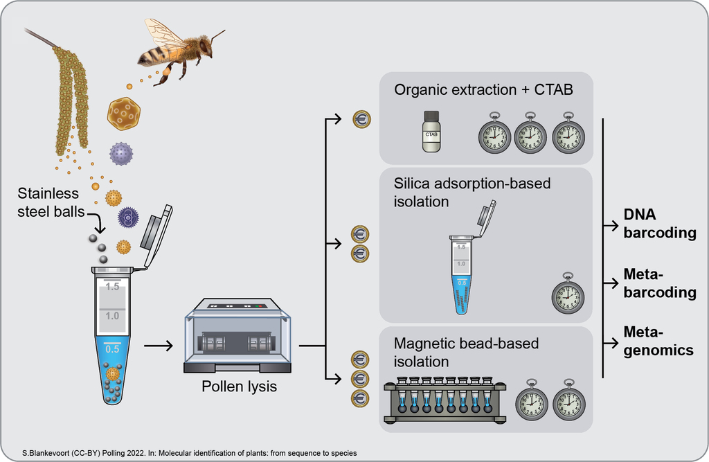
Chapter 5 Infographic: Overview of pollen sources, DNA extraction, and downstream analytical methods for the molecular identification of plants from pollen DNA.
While research into targeting different barcoding regions and primers is ongoing (trnT-F;
It is important to use positive controls with known concentrations of different pollen species in any DNA metabarcoding study. This is because the amount of DNA that can be extracted from different pollen types has been shown to vary. For example, it can be easier to extract DNA from pollen with a thinner exine and from plant species that are richer in chloroplast DNA than from those having a more ‘sturdy’ exine (
Quantitative pollen analysis
Beyond identifying which pollen species are present in a particular sample, pollen grain quantification is equally important. For example, for hay fever forecasts, it is not just important to know if there are certain allergenic pollen in the air, but also how many pollen grains there are at a given point in time. The golden standard for palynology has been to count a certain number of pollen grains under the microscope (e.g., 200 to 500) to obtain a semi-quantitative measure of the pollen types in a sample. While DNA-based methods for pollen quantification are less developed than DNA-based methods for identification, DNA-based pollen quantification using metagenomics (reviewed in Chapter 12 Metagenomics) seems feasible, while there is still strong debate about using DNA metabarcoding reads for this purpose.
DNA metabarcoding reads
In a recent study on the use of DNA to quantify pollen grains, Bell and colleagues found a very weak correlation between pollen counts recorded by palynologists and the proportion of metabarcoding reads (
Another group of scholars, however, are finding more promising results in using DNA metabarcoding to quantify pollen grains.
Metagenomic approaches
Since using DNA metabarcoding approaches for pollen abundance may not give quantitative results with complex, multi-species samples, other molecular methods such as genome skimming and shotgun sequencing are being used to circumvent some of the drawbacks. The major advantage of these two methods is that they do not include a PCR-step and therefore do not introduce amplification bias (see Chapter 12 Metagenomics). Genome skimming has already been used to show that quantification is feasible, even for pollen from species that are very rare in mock mixtures (
Questions
- What are the main advantages of molecular pollen identification over traditional (microscopic) methods? Justify your answer.
- Pollen is dispersed by various vectors. There are two main types of pollination strategies in land plants, please name them and also explain the importance of the difference between the two in terms of DNA yield.
- Which four factors make the quantification of pollen grains using metabarcoding problematic?
Glossary
Anemophilous – Wind-pollinated.
Bead beating – The application of beads to break open the outer cell wall of pollen grains.
Hirst-type pollen trap – Volumetric air sampler that is one of the standard devices for monitoring airborne pollen and spores.
cpDNA – Chloroplast DNA.
Entomophilous – Insect-pollinated.
Exine – Outer wall of pollen grains. Composed mainly of sporopollenin that is extremely resistant to degradation. The exine of pollen grains has to be broken to release the DNA from the organic material within the grains.
Palynology – The science that studies both living and fossil spores, pollen grains, and other microscopic structures (e.g., chironomids, dinocysts, acritarchs, chitinozoans, scolecodonts).
Pollen grains – The male gametophyte of seed plants; source and carrier for the male gametes (spermatozoids or sperm cells).
Pollenkitt – The outermost hydrophobic lipid layer mostly present on entomophilous pollen grains.
Sporopollenin – A chemically inert biological polymer that is a component of the outer wall (see Exine) of a pollen grain.
Super-resolution microscopy – Technique in optical microscopy that allows visualisation of images with resolutions up to 140 nm, much higher than those imposed by the diffraction limit. This technique also allows visualisation of internal structures.
References
- Alan Ş, Sarışahin T, Şahin AA, Kaplan A, Erdoğan İ, Pınar NM (2019) A new method to quantify atmospheric Poaceae pollen DNA based on the trnT-F cpDNA region. Turk. J. Bioch. 44, 248–253. doi: 10.1515/tjb-2018-0020
- Baksay S, Pornon A, Burrus M, Mariette J, Andalo C, Escaravage N (2020) Experimental quantification of pollen with DNA metabarcoding using ITS1 and trnL. Sci. Rep. 10, 4202. doi: 10.1038/s41598-020-61198-6
- Banchi E, Pallavicini A, Muggia L (2020) Relevance of plant and fungal DNA metabarcoding in aerobiology. Aerobiologia (Bologna) 36, 9–23. doi: 10.1007/s10453-019-09574-2
- Bänsch S, Tscharntke T, Wünschiers R, Netter L, Brenig B, Gabriel D, Westphal C (2020) Using ITS2 metabarcoding and microscopy to analyse shifts in pollen diets of honey bees and bumble bees along a mass-flowering crop gradient. Mol. Ecol. 29, 5003–5018. doi: 10.1111/mec.15675
- Bell KL, Burgess KS, Botsch JC, Dobbs EK, Read TD, Brosi BJ (2019) Quantitative and qualitative assessment of pollen DNA metabarcoding using constructed species mixtures. Mol. Ecol. 28, 431–455. doi: 10.1111/mec.14840
- Bell KL, Burgess KS, Okamoto KC, Aranda R, Brosi BJ (2016a) Review and future prospects for DNA barcoding methods in forensic palynology. Forensic Sci. Int. Genet. 21, 110–116. doi: 10.1016/j.fsigen.2015.12.010
- Bell KL, de Vere N, Keller A, Richardson RT, Gous A, Burgess KS, Brosi BJ (2016b) Pollen DNA barcoding: current applications and future prospects. Genome 59, 629–640. doi: 10.1139/gen-2015-0200
- Bell KL, Fowler J, Burgess KS, Dobbs EK, Gruenewald D, Lawley B, Morozumi C, Brosi BJ (2017) Applying pollen DNA metabarcoding to the study of plant-pollinator interactions. Appl. Plant Sci. 5, 1600124. doi: 10.3732/apps.1600124
- Beug H-J (2004) Leitfaden der Pollenbestimmung für Mitteleuropa und angrenzende Gebiete. Friedrich Pfeil, München.
- Brennan GL, Potter C, de Vere N, Griffith GW, Skjøth CA, Osborne NJ, Wheeler BW, McInnes RN, Clewlow Y, Barber A, Hanlon HM, Hegarty M, Jones L, Kurganskiy A, Rowney FM, Armitage C, Adams-Groom B, Ford CR, Petch GM, PollerGEN Consortium Creer S (2019) Temperate airborne grass pollen defined by spatio-temporal shifts in community composition. Nat. Ecol. Evol. 3, 750–754. doi: 10.1038/s41559-019-0849-7
- Brooks J, Shaw G (1968) Chemical structure of the exine of pollen walls and a new function for carotenoids in nature. Nature 219, 532–533. doi: 10.1038/219532a0
- Campbell BC, Al Kouba J, Timbrell V, Noor MJ, Massel K, Gilding EK, Angel N, Kemish B, Hugenholtz P, Godwin ID, Davies JM (2020) Tracking seasonal changes in diversity of pollen allergen exposure: Targeted metabarcoding of a subtropical aerobiome. Sci. Total Environ. 747, 141189. doi: 10.1016/j.scitotenv.2020.141189
- Deagle BE, Thomas AC, McInnes JC, Clarke LJ, Vesterinen EJ, Clare EL, Kartzinel TR, Eveson JP (2019) Counting with DNA in metabarcoding studies: how should we convert sequence reads to dietary data? Mol. Ecol. 28, 391–406. doi: 10.1111/mec.14734
- Frenguelli G, Passalacqua G, Bonini S, Fiocchi A, Incorvaia C, Marcucci F, Tedeschini E, Canonica GW, Frati F (2010) Bridging allergologic and botanical knowledge in seasonal allergy: a role for phenology. Ann. Allergy Asthma Immunol. 105, 223–227. doi: 10.1016/j.anai.2010.06.016
- Ghitarrini S, Pierboni E, Rondini C, Tedeschini E, Tovo GR, Frenguelli G, Albertini E (2018) New biomolecular tools for aerobiological monitoring: Identification of major allergenic Poaceae species through fast real-time PCR. Ecol. Evol. 8, 3996–4010. doi: 10.1002/ece3.3891
- Gous A, Swanevelder DZH, Eardley CD, Willows-Munro S (2019) Plant-pollinator interactions over time: Pollen metabarcoding from bees in a historic collection. Evol. Appl. 12, 187–197. doi: 10.1111/eva.12707
- Hawkins J, de Vere N, Griffith A, Ford CR, Allainguillaume J, Hegarty MJ, Baillie L, Adams-Groom B (2015) Using DNA metabarcoding to identify the floral composition of honey: A new tool for investigating honey bee foraging preferences. PLoS ONE 10, e0134735. doi: 10.1371/journal.pone.0134735
- Hirst JM (1952) AN AUTOMATIC VOLUMETRIC SPORE TRAP. Ann. Applied Biology 39, 257–265. doi: 10.1111/j.1744-7348.1952.tB010500904.x
- Hochuli PA, Feist-Burkhardt S (2013) Angiosperm-like pollen and Afropollis from the Middle Triassic (Anisian) of the Germanic Basin (Northern Switzerland). Front. Plant Sci. 4, 344. doi: 10.3389/fpls.2013.00344
- Hollingsworth PM (2011) Refining the DNA barcode for land plants. Proc Natl Acad Sci USA 108, 19451–19452. doi: 10.1073/pnas.1116812108
- Kraaijeveld K, de Weger LA, Ventayol García M, Buermans H, Frank J, Hiemstra PS, den Dunnen JT (2015) Efficient and sensitive identification and quantification of airborne pollen using next-generation DNA sequencing. Mol. Ecol. Resour. 15, 8–16. doi: 10.1111/1755-0998.12288
- Lamb PD, Hunter E, Pinnegar JK, Creer S, Davies RG, Taylor MI (2019) How quantitative is metabarcoding: A meta-analytical approach. Mol. Ecol. 28, 420–430. doi: 10.1111/mec.14920
- Lang D, Tang M, Hu J, Zhou X (2019) Genome-skimming provides accurate quantification for pollen mixtures. Mol. Ecol. Resour. 19, 1433–1446. doi: 10.1111/1755-0998.13061
- Leidenfrost RM, Bänsch S, Prudnikow L, Brenig B, Westphal C, Wünschiers R (2020) Analyzing the dietary diary of bumble bee. Front. Plant Sci. 11, 287. doi: 10.3389/fpls.2020.00287
- Leontidou K, Vernesi C, De Groeve J, Cristofolini F, Vokou D, Cristofori A (2018) DNA metabarcoding of airborne pollen: new protocols for improved taxonomic identification of environmental samples. Aerobiologia (Bologna) 34, 63–76. doi: 10.1007/s10453-017-9497-z
- Levetin E (2004) Methods for aeroallergen sampling. Curr. Allergy Asthma Rep. 4, 376–383. doi: 10.1007/s11882-004-0088-z
- Meiklejohn KA, Damaso N, Robertson JM (2019) Assessment of BOLD and GenBank - Their accuracy and reliability for the identification of biological materials. PLoS ONE 14, e0217084. doi: 10.1371/journal.pone.0217084
- Mohanty RP, Buchheim MA, Levetin E (2017) Molecular approaches for the analysis of airborne pollen: A case study of Juniperus pollen. Ann. Allergy Asthma Immunol. 118, 204-211.e2. doi: 10.1016/j.anai.2016.11.015
- Müller-Germann I, Pickersgill DA, Paulsen H, Alberternst B, Pöschl U, Fröhlich-Nowoisky J, Després VR (2017) Allergenic Asteraceae in air particulate matter: quantitative DNA analysis of mugwort and ragweed. Aerobiologia (Bologna) 33, 493–506. doi: 10.1007/s10453-017-9485-3
- Pacini E, Hesse M (2005) Pollenkitt – its composition, forms and functions. Flora - Morphology, Distribution, Functional Ecology of Plants 200, 399–415. doi: 10.1016/j.flora.2005.02.006
- Parducci L, Bennett KD, Ficetola GF, Alsos IG, Suyama Y, Wood JR, Pedersen MW (2017) Ancient plant DNA in lake sediments. New Phytol. 214, 924–942. doi: 10.1111/nph.14470
- Pawluczyk M, Weiss J, Links MG, Egaña Aranguren M, Wilkinson MD, Egea-Cortines M (2015) Quantitative evaluation of bias in PCR amplification and next-generation sequencing derived from metabarcoding samples. Anal. Bioanal. Chem. 407, 1841–1848. doi: 10.1007/s00216-014-8435-y
- Peel N, Dicks LV, Clark MD, Heavens D, Percival-Alwyn L, Cooper C, Davies RG, Leggett RM, Yu DW (2019) Semi-quantitative characterisation of mixed pollen samples using MinION sequencing and Reverse Metagenomics (RevMet). Methods Ecol. Evol. 10, 1690–1701. doi: 10.1111/2041-210X.13265
- Polling M, Li C, Cao L, Verbeek F, de Weger LA, Belmonte J, De Linares C, Willemse J, de Boer H, Gravendeel B (2021) Neural networks for increased accuracy of allergenic pollen monitoring. Sci. Rep. 11, 11357. doi: 10.1038/s41598-021-90433-x
- Pornon A, Andalo C, Burrus M, Escaravage N (2017) DNA metabarcoding data unveils invisible pollination networks. Sci. Rep. 7, 16828. doi: 10.1038/s41598-017-16785-5
- Prosser SWJ, Hebert PDN (2017) Rapid identification of the botanical and entomological sources of honey using DNA metabarcoding. Food Chem. 214, 183–191. doi: 10.1016/j.foodchem.2016.07.077
- Richardson RT, Curtis HR, Matcham EG, Lin C-H, Suresh S, Sponsler DB, Hearon LE, Johnson RM (2019) Quantitative multi-locus metabarcoding and waggle dance interpretation reveal honey bee spring foraging patterns in Midwest agroecosystems. Mol. Ecol. 28, 686–697. doi: 10.1111/mec.14975
- Richardson RT, Lin C-H, Sponsler DB, Quijia JO, Goodell K, Johnson RM (2015) Application of ITS2 metabarcoding to determine the provenance of pollen collected by honey bees in an agroecosystem. Appl. Plant Sci. 3, 1400066. doi: 10.3732/apps.1400066
- Romero IC, Kong S, Fowlkes CC, Jaramillo C, Urban MA, Oboh-Ikuenobe F, D’Apolito C, Punyasena SW (2020) Improving the taxonomy of fossil pollen using convolutional neural networks and superresolution microscopy. Proc. Natl. Acad. Sci. USA 17, 28496–28505. doi: 10.1073/pnas.2007324117
- Sivaguru M, Urban MA, Fried G, Wesseln CJ, Mander L, Punyasena SW (2018) Comparative performance of airyscan and structured illumination superresolution microscopy in the study of the surface texture and 3D shape of pollen. Microsc. Res. Tech. 81, 101–114. doi: 10.1002/jemt.22732
- Suchan T, Talavera G, Sáez L, Ronikier M, Vila R (2019) Pollen metabarcoding as a tool for tracking long-distance insect migrations. Mol. Ecol. Resour. 19, 149–162. doi: 10.1111/1755-0998.12948
- Suyama Y, Kawamuro K, Kinoshita I, Yoshimura K, Tsumura Y, Takahara H (1996) DNA sequence from a fossil pollen of Abies spp. from Pleistocene peat. Genes Genet. Syst. 71, 145–149. doi: 10.1266/ggs.71.145
- Swenson SJ, Gemeinholzer B (2021) Testing the effect of pollen exine rupture on metabarcoding with Illumina sequencing. PLoS ONE 16, e0245611. doi: 10.1371/journal.pone.0245611
- Utzeri VJ, Schiavo G, Ribani A, Tinarelli S, Bertolini F, Bovo S, Fontanesi L (2018) Entomological signatures in honey: an environmental DNA metabarcoding approach can disclose information on plant-sucking insects in agricultural and forest landscapes. Sci. Rep. 8, 9996. doi: 10.1038/s41598-018-27933-w
Answers
- A higher taxonomic resolution can be achieved using molecular methods such as metabarcoding. Furthermore, pollen analysis requires highly trained experts that have to spend considerable time to analyse a single sample and therefore molecular techniques are faster, especially with a large number of samples.
- Entomophilous (insect collected) and anemophilous (wind dispersed) pollen. The presence of pollenkitt on entomophilous pollen grains influences the amount of DNA that can be obtained per pollen grain.
- Copy number, DNA preservation, DNA isolation technique, and amplification bias.
Chapter 6 DNA from food and medicine
Why use DNA for the identification of food and medicine?
DNA-based methods for the molecular identification of plant products can help us to address food and medicine authenticity issues at each stage in the supply chain (Di Bernardo et al. 2007). Documentation and requirements for DNA-based detection methods for food authentication are defined in collaborative activities by the European Committee for Standardization (CEN) and the International Organization for Standardization (ISO). Both rapid and accurate identification of plant products are crucial for the the herbal drug industry (
DNA-based methods to identify plants in food and medicine
The majority of standardised DNA-based authentication methods for the inspection and regulation of food and plant-medicines use well-established PCR-based techniques for DNA amplification as these are sensitive, specific, and simple (
DNA barcoding methods are also established for the identification of unique medicinal and edible plant species (
High-throughput sequencing (HTS) methods such as amplicon metabarcoding are also powerful tools for the authentication of herbal end products, post-marketing control, pharmacovigilance, and the assessment of species composition in botanical medicines, such as in traditional Chinese medicines (TCMs) (
In addition to PCR-based techniques, the detection of single nucleotide polymorphisms (SNPs) is frequently used for the molecular identification and authentication of various food commodities using small DNA fragments (Di Bernardo et al. 2007;
DNA-based methods for molecular plant identification depend on well-curated nucleotide sequence repositories. In addition to GenBank (
DNA isolation from food and medicines
Successful DNA extraction is the foundation for any further downstream analysis (
Factors affecting the efficacy of DNA extraction
Four main factors that affect the efficacy of DNA isolation from food and medicine samples are the sample source and processing, collection and storage, homogenisation, and the presence of contaminants. Generally it is easier to extract high-quality DNA from fresh samples (
Removal of frequent contaminants that can reduce the yield of extracted DNA from edible and medicinal plants.
| Proteins and RNA | |||
|---|---|---|---|
| What compounds define the chemical composition of your samples? | Polysaccharides (starch, sugars) | Polyphenolics | |
| RNA | (plant secondary metabolites like: tannins, flavonoids, terpenoids, etc.) | ||
| Understand the specific properties of your samples for DNA extraction | Can co-purify with DNA | Can co-precipitate with DNA | When bound to DNA very hard to remove in extraction |
| dependending on the age of the samples and how they were conserved | Results in a sticky viscous consistency to DNA pellet after centrifugation | ||
| Inhibition of enzymes used for molecular techniques (restriction endonucleases, polymerases, and ligases ( |
Results in contaminated pellets not usable for many downstream analyses ( |
||
| Adherence to wells in agarose gel residing in long smears of bands detected in gel ( |
|||
| Consider applying mitigation strategies to overcome difficulties in extracting DNA from your samples | RNA removable with DNase-free RNase A or ethanol precipitation using lithium chloride | Removal via highly concentrated sodium chloride (NaCl) in extraction buffers leading to increased solubility in ethanol | Binder compounds polyvinyl pyrrolidone (PVP) or polypyrrolidone (PVPP) can be used in extraction buffers to absorb polyphenols before polymerization with DNA |
| Proteins can be removed by i) inclusion of detergents (cetyltrimethylammonium bromide (CTAB), SDS) in extraction buffer | |||
| Combination of NaCl and cationic detergent CTAB | |||
| CTAB with differential precipitation ( |
|||
| Use of antioxidant compounds (BME, DDT, ascorbic acid, iso-ascorbate) in buffer to prevent polymerization ( |
|||
| ii) protein denaturants e.g., β-mercaptoethanol (BME), dithiothreitol (DTT) | |||
| iii) enzymatic proteases e.g., proteinase K | |||
Although CTAB-based methods usually result in DNA extraction from plants and processed food and medicine products, the quantity is often quite low and the protocols are time consuming (
Commercial vs. in-house DNA isolation techniques
Several studies exist that compare commercial and in-house DNA isolation techniques for food and medicine (
Overview of different DNA extraction methods recommended for use with food by the European Union Reference Laboratory for GM Food and Feed (EU-RL GMFF).
| Plant source | Method of choice | Reference |
|---|---|---|
| Maize | CTAB precipitate (in-house) (Rogers and Bendich 1985) | CRLVL16/05XP corrected version 2 01/03/2018 |
| Maize seeds and grains | For isolation of genomic DNA from a wide variety of maize tissues and derived matrices for high-quality genomic DNA from processed plant tissue (e.g., leaf, grain, or seed). | |
| Lysis step (thermal lysis in the presence of Tris HCl, EDTA, CTAB, and β-mercaptoethanol). | ||
| Tissues processed prior to extraction procedure. Possible methods of processing include a mortar and pestle with liquid nitrogen (leaf) or commercial blender (grain or seed). | ||
| Soybean | CTAB precipitate (in-house) (Dellaporta et al. 1983) | CRLVL13/05XP 14/05/2007 |
| Soybean seeds | “Dellaporta-derived” method starts with a lysis step (thermal lysis in the presence of Tris HCl, EDTA, NaCl, and β-mercaptoethanol). | |
| Isopropanol precipitation and removal of contaminants such as lipophilic molecules and proteins by extraction with phenol:chloroform:isoamyl alcohol. | ||
| Potato | “CTAB/Microspin” method | CRLVL09/05XP Corrected Version 1 20/01/2009 |
| Freeze-dried potato tubers | Lysis step (thermal lysis in the presence of CTAB, EDTA, and proteinase K). | |
| Removal of RNA by digestion with RNase A and removal of contaminants such as lipophilic molecules and proteins by extraction with chloroform. | ||
| Remaining inhibitors are removed by a gel filtration step using the commercially available product S-300 HR Microspin Columns (Amersham Pharmacia). | ||
| Rapeseed | CTAB precipitate (in-house) (Dellaporta et al. 1983) | CRLVL14/04XP Corrected Version 1 15/01/2007 |
| Lysis step (thermal lysis in the presence of Tris HCl, EDTA, SDS, and β-mercaptoethanol). | ||
| Removal of contaminants such as lipophilic molecules and proteins by extraction with phenol and chloroform. | ||
| DNA precipitate is generated by using isopropanol. The pellet is dissolved in TE buffer. | ||
| Rapeseed | Inhibitors are removed by an anion exchange chromatography step using the DNA Clean & Concentrator 25 kit (Zymo Research). | CRLVL14/04XP Corrected Version 1 15/01/2007 |
| Multi-herbal products | CTAB precipitate (in-house) (Murray and Thompson 1980) | Arulandhu et al. 2017 |
| Technique is ideal for the rapid isolation of small amounts of DNA from many different species and is also useful for large scale isolations. | ||
| Lysis step (thermal lysis in the presence of Tris HCl, EDTA, CTAB, and β-mercaptoethanol). | ||
| Removal of contaminants such as lipophilic molecules and proteins by extraction with phenol and chloroform. | ||
| Samples processed prior to extraction procedure (mortar and pestle, liquid nitrogen, or commercial blender). |
Analysing the quantity and purity of extracted DNA
After DNA extraction, measuring both the DNA concentration and purity is important before continuing with further downstream analysis. Isolated DNA can be tested for quality using absorbance methods, agarose gel electrophoresis, and fluorescent DNA-intercalating dyes (
The reality of DNA-based identification
It is in the interest of both biodiversity conservation and public safety that DNA-based techniques are further developed to screen food and medicine sourced from the global market (
Questions
- The quality of DNA from food and medicinal sources is a critical factor for DNA-based analyses. Which factors can influence the quality of nucleic acids extracted from foods and plant-based medicines?
- What is the first step when choosing a DNA isolation technique for your samples?
- What methods can be used for measuring DNA quality after isolation?
Glossary
Bioprospecting - The exploration of biodiversity for new resources of social and commercial value.
Pharmacophylogenomics - Plant pharmacophylogenomics is a field established by combining the fields of ethnopharmacology, plant systematics, phytochemistry, pharmacology, and bioinformatics. It is the application of phylogenomics to the study of pharmaceuticals.
Pharmacopoeia - From the obsolete typography pharmacopœia, literally, “drug-making”. In its modern technical sense, it is a book containing directions for the identification of compound medicines, and is published by the authority of a government or a medical or pharmaceutical society.
Pharmaphylogenetics - Field of research focusing on the phylogenetic correlation between phylogeny, chemical constituents, and pharmaceutical effects of medicinal plants.
References
- Arulandhu AJ, Staats M, Hagelaar R, Voorhuijzen MM, Prins TW, Scholtens I, Costessi A, Duijsings D, Rechenmann F, Gaspar FB, Barreto Crespo MT, Holst-Jensen A, Birck M, Burns M, Haynes E, Hochegger R, Klingl A, Lundberg L, Natale C, Niekamp H, Kok E (2017) Development and validation of a multi-locus DNA metabarcoding method to identify endangered species in complex samples. Gigascience 6, 1–18. doi: 10.1093/gigascience/gix080
- Benson DA, Cavanaugh M, Clark K, Karsch-Mizrachi I, Ostell J, Pruitt KD, Sayers EW (2018) GenBank. Nucleic Acids Res. 46, D41–D47. doi: 10.1093/nar/gkx1094
- Boom R, Sol CJ, Salimans MM, Jansen CL, Wertheim-van Dillen PM, van der Noordaa J (1990) Rapid and simple method for purification of nucleic acids. J. Clin. Microbiol. 28, 495–503. doi: 10.1128/jcm.28.3.495-503.1990
- British Pharmacopoeia Commission (2018) Supplementary chapter SC VII D, in: DNA Barcoding as a Tool for Botanical Identification of Herbal Drugs. The Stationary Office, London, United Kingdom.
- Coghlan ML, Haile J, Houston J, Murray DC, White NE, Moolhuijzen P, Bellgard MI, Bunce M (2012) Deep sequencing of plant and animal DNA contained within traditional Chinese medicines reveals legality issues and health safety concerns. PLoS Genet. 8, e1002657. doi: 10.1371/journal.pgen.1002657
- Corrado G (2016) Advances in DNA typing in the agro-food supply chain. Trends Food Sci. Technol. 52, 80–89. doi: 10.1016/j.tifs.2016.04.003
- Costa J, Amaral JS, Fernandes TJR, Batista A, Oliveira MBPP, Mafra I (2015) DNA extraction from plant food supplements: influence of different pharmaceutical excipients. Mol. Cell. Probes 29, 473–478. doi: 10.1016/j.mcp.2015.06.002
- Dellaporta SL, Wood J, Hicks JB (1983) A plant DNA minipreparation: Version II. Plant Mol. Biol. Rep. 1, 19–21. doi: 10.1007/BF010602712670
- De Boer HJ, Cross HB, De Wilde WJJO, Duyfjes-de Wilde BEE, Gravendeel B (2015) Molecular phylogenetic analyses of Cucurbitaceae tribe Benincaseae urge for merging of Pilogyne with Zehneria. Phytotaxa 236, 173. doi: 10.11646/phytotaxa.236.2.6
- Di Bernardo G, Del Gaudio S, Galderisi U, Cascino A, Cipollaro M (2007) Comparative evaluation of different DNA extraction procedures from food samples. Biotechnol. Prog. 23, 297–301. doi: 10.1021/bp060182m
- Elsanhoty RM, Ramadan MF, Jany KD (2011) DNA extraction methods for detecting genetically modified foods: a comparative study. Food Chem. 126, 1883–1889. doi: 10.1016/j.foodchem.2010.12.013
- Grazina L, Amaral JS, Mafra I (2020) Botanical origin authentication of dietary supplements by DNA-based approaches. Comp. Rev. Food Sci. Food Safety 19, 1080–1109. doi: 10.1111/1541-4337.12551
- Grohmann L, Seiler C (2019) CHAPTER 21. Standardization of DNA-based Methods for Food Authenticity Testing, in: Burns, M., Foster, L., Walker, M. (Eds.), DNA Techniques to Verify Food Authenticity: Applications in Food Fraud, Food Chemistry, Function and Analysis. Royal Society of Chemistry, Cambridge, pp. 227–234. doi: 10.1039/9781788016025-00227
- Gryson N, Messens K, Dewettinck K (2004) Evaluation and optimisation of five different extraction methods for soy DNA in chocolate and biscuits. Extraction of DNA as a first step in GMO analysis. J. Sci. Food Agric. 84, 1357–1363. doi: 10.1002/jsfa.1767
- Gryson N (2010) Effect of food processing on plant DNA degradation and PCR-based GMO analysis: a review. Anal. Bioanal. Chem. 396, 2003–2022. doi: 10.1007/s00216-009-3343-2
- Han J, Pang X, Liao B, Yao H, Song J, Chen S (2016) An authenticity survey of herbal medicines from markets in China using DNA barcoding. Sci. Rep. 6, 18723. doi: 10.1038/srep18723
- Hao D, Xiao P, Liu L, Peng Y, He C (2015) [Essentials of pharmacophylogeny: knowledge pedigree, epistemology and paradigm shift]. Zhongguo Zhong Yao Za Zhi 40, 3335–3342.
- Hirst B, Fernandez-Calvino L, Weiss T (2019) Chapter 24. Commercial DNA testing, in: Burns, M., Foster, L., Walker, M. (Eds.), DNA Techniques to Verify Food Authenticity: Applications in Food Fraud, Food Chemistry, Function and Analysis. Royal Society of Chemistry, Cambridge, pp. 264–282. doi: 10.1039/9781788016025-00264
- Hoorfar J, Cook N, Malorny B, Wagner M, De Medici D, Abdulmawjood A, Fach P (2004) Letter to the editor. Lett. Appl. Microbiol. 38, 79–80. doi: 10.1046/j.1472-765X.2003.01456.x
- Howard C, Lockie-Williams C, Slater A (2020) Applied barcoding: the practicalities of DNA testing for herbals. Plants 9. doi: 10.3390/plants9091150
- Ichim MC, de Boer HJ (2020) A review of authenticity and authentication of commercial ginseng herbal medicines and food supplements. Front. Pharmacol. 11, 612071. doi: 10.3389/fphar.2020.612071
- Ichim MC (2019) The DNA-based authentication of commercial herbal products reveals their globally widespread adulteration. Front. Pharmacol. 10, 1227. doi: 10.3389/fphar.2019.01227
- John ME (1992) An efficient method for isolation of RNA and DNA from plants containing polyphenolics. Nucleic Acids Res. 20, 2381. doi: 10.1093/nar/20.9.2381
- Juul S, Izquierdo F, Hurst A, Dai X, Wright A, Kulesha E, Pettett R, Turner DJ (2015) What’s in my pot? Real-time species identification on the MinION. BioRxiv. doi: 10.1101/030742
- Llongueras JP, Nair S, Salas-Leiva D, Schwarzbach AE (2013) Comparing DNA extraction methods for analysis of botanical materials found in anti-diabetic supplements. Mol. Biotechnol. 53, 249–256. doi: 10.1007/s12033-012-9520-0
- Lockley AK, Bardsley RG (2000) DNA-based methods for food authentication. Trends Food Sci. Technol. 11, 67–77. doi: 10.1016/S0924-2244(00)00049-2
- Lo Y-T, Shaw P-C (2018a) DNA-based techniques for authentication of processed food and food supplements. Food Chem. 240, 767–774. doi: 10.1016/j.foodchem.2017.08.022
- Lo Y-T, Shaw P-C (2018b) DNA barcoding in concentrated Chinese medicine granules using adaptor ligation-mediated polymerase chain reaction. J. Pharm. Biomed. Anal. 149, 512–516. doi: 10.1016/j.jpba.2017.11.048
- Lo YT, Shaw PC (2019) Application of next-generation sequencing for the identification of herbal products. Biotechnol. Adv. 37, 107450. doi: 10.1016/j.biotechadv.2019.107450
- Matsuoka T, Kuribara H, Akiyama H, Miura H, Goda Y, Kusakabe Y, Isshiki K, Toyoda M, Hino A (2001) A multiplex PCR method of detecting recombinant DNAs from five lines of genetically modified maize. Shokuhin Eiseigaku Zasshi 42, 24–32. doi: 10.3358/shokueishi.42.24
- Mezzasalma V, Ganopoulos I, Galimberti A, Cornara L, Ferri E, Labra M (2017) Poisonous or non-poisonous plants? DNA-based tools and applications for accurate identification. Int. J. Legal Med. 131, 1–19. doi: 10.1007/s00414-016-1460-y
- Mishra P, Kumar A, Nagireddy A, Mani DN, Shukla AK, Tiwari R, Sundaresan V (2016) DNA barcoding: an efficient tool to overcome authentication challenges in the herbal market. Plant Biotechnol. J. 14, 8–21. doi: 10.1111/pbi.12419
- Murray MG, Thompson WF (1980) Rapid isolation of high molecular weight plant DNA. Nucleic Acids Res. 8, 4321–4325. doi: 10.1093/nar/8.19.4321
- Omelchenko DO, Speranskaya AS, Ayginin AA, Khafizov K, Krinitsina AA, Fedotova AV, Pozdyshev DV, Shtratnikova VY, Kupriyanova EV, Shipulin GA, Logacheva MD (2019) Improved Protocols of ITS1-Based Metabarcoding and Their Application in the Analysis of Plant-Containing Products. Genes (Basel) 10. doi: 10.3390/genes10020122
- Pafundo S, Gullì M, Marmiroli N (2011) Comparison of DNA extraction methods and development of duplex PCR and real-time PCR to detect tomato, carrot, and celery in food. J. Agric. Food Chem. 59, 10414–10424. doi: 10.1021/jF0106202382s
- Pandey RN, Adams RP, Flournoy LE (1996) Inhibition of random amplified polymorphic DNAs (RAPDs) by plant polysaccharides. Plant Mol. Biol. Rep. 14, 17–22. doi: 10.1007/BF010602671898
- Parveen I, Gafner S, Techen N, Murch SJ, Khan IA (2016) DNA barcoding for the identification of botanicals in herbal medicine and dietary supplements: strengths and limitations. Planta Med. 82, 1225–1235. doi: 10.1055/s-0042-111208
- Pawar RS, Handy SM, Cheng R, Shyong N, Grundel E (2017) Assessment of the authenticity of herbal dietary supplements: comparison of chemical and DNA barcoding methods. Planta Med. 83, 921–936. doi: 10.1055/s-0043-107881
- Peterson DG, Boehm KS, Stack SM (1997) Isolation of milligram quantities of nuclear DNA from tomato (Lycopersicon esculentum), A plant containing high levels of polyphenolic compounds. Plant Mol. Biol. Rep. 15, 148–153. doi: 10.1007/BF010602812265
- Pharmacopoeia Committee of P. R. China (2020) Pharmacopoeia of People’s Republic of China. China Medical Science and Technology Press, Beijing.
- Pich U, Schubert I (1993) Midiprep method for isolation of DNA from plants with a high content of polyphenolics. Nucleic Acids Res. 21, 3328. doi: 10.1093/nar/21.14.3328
- Pinto AD, Forte V, Guastadisegni MC, Martino C, Schena FP, Tantillo G (2007) A comparison of DNA extraction methods for food analysis. Food Control 18, 76–80. doi: 10.1016/j.foodcont.2005.08.011
- Puchooa D (2004) A simple, rapid and efficient method for the extraction of genomic DNA from lychee (Litchi chinensis Sonn.). Afr. J. Biotechnol. 3, 253–255. doi: 10.5897/AJB01062004.000-2046
- Raclariu AC, Heinrich M, Ichim MC, de Boer H (2018) Benefits and limitations of DNA barcoding and metabarcoding in herbal product authentication. Phytochem. Anal. 29, 123–128. doi: 10.1002/pca.2732
- Raime K, Krjutškov K, Remm M (2020) Method for the Identification of Plant DNA in Food Using Alignment-Free Analysis of Sequencing Reads: A Case Study on Lupin. Front. Plant Sci. 11, 646. doi: 10.3389/fpls.2020.00646
- Ratnasingham S, Hebert PDN (2007) BOLD: The Barcode of Life Data System (http://www.barcodinglife.org). Mol. Ecol. Notes 7, 355–364. doi: 10.1111/j.1471-8286.2007.01678.x
- Rogers SO, Bendich AJ (1985) Extraction of DNA from milligram amounts of fresh, herbarium and mummified plant tissues. Plant Mol. Biol. 5, 69–76. doi: 10.1007/BF010600020088
- Seethapathy GS, Raclariu-Manolica A-C, Anmarkrud JA, Wangensteen H, de Boer HJ (2019) DNA metabarcoding authentication of ayurvedic herbal products on the European market raises concerns of quality and fidelity. Front. Plant Sci. 10, 68. doi: 10.3389/fpls.2019.00068
- Sharma AD, Gill PK, Singh P (2002) DNA isolation from dry and fresh samples of polysaccharide-rich plants. Plant Mol. Biol. Rep. 20, 415–415. doi: 10.1007/BF010602772129
- Smith DS, Maxwell PW, De Boer SH (2005) Comparison of several methods for the extraction of DNA from potatoes and potato-derived products. J. Agric. Food Chem. 53, 9848–9859. doi: 10.1021/jF0106051201v
- Techen N, Parveen I, Pan Z, Khan IA (2014) DNA barcoding of medicinal plant material for identification. Curr. Opin. Biotechnol. 25, 103–110. doi: 10.1016/j.copbio.2013.09.010
- Turkec A, Kazan H, Karacanli B, Lucas SJ (2015) DNA extraction techniques compared for accurate detection of genetically modified organisms (GMOs) in maize food and feed products. J. Food Sci. Technol. 52, 5164–5171. doi: 10.1007/s13197-014-1547-8
- Unable to find information for 9645779, n.d.
- Wilkes T (2019) CHAPTER 3. DNA Extraction from Food Matrices, in: Burns, M., Foster, L., Walker, M. (Eds.), DNA Techniques to Verify Food Authenticity: Applications in Food Fraud, Food Chemistry, Function and Analysis. Royal Society of Chemistry, Cambridge, pp. 29–49. doi: 10.1039/9781788016025-00029
- Wong T-H, But GW-C, Wu H-Y, Tsang SS-K, Lau DT-W, Shaw P-C (2018) Medicinal Materials DNA Barcode Database (MMDBD) version 1.5-one-stop solution for storage, BLAST, alignment and primer design. Database (Oxford) 2018. doi: 10.1093/database/bay112
- Wood EJ (2002) Principles and techniques of practical biochemistry (5th Ed.): Wilson, K., Walker, J. (eds.). Biochem. Mol. Biol. Educ. 30, 214–215. doi: 10.1002/bmb.2002.494030030062
Answers
- Sample source and processing, collection and storage, homogenisation, and the presence of contaminants.
- One should firstly consider whether it is a complex mixture or a pure product, and the degree of processing (form and degree of homogeneity).
- Absorbance methods, agarose gel electrophoresis, and fluorescent DNA-intercalating dyes.
Chapter 7 DNA from faeces
Background
What are faecal samples?
Do you know that faeces are windows to the natural world? Faeces, although not the most glamorous thing in the world, are worth their weight in gold when it comes to providing information about the host(s) they are derived from. Faeces, also commonly known as scat, poop, droppings, excreta, or stools are solid remains of the ingested food that were not digested in the intestine. They are composed of water, protein, polysaccharides, fats, solids (e.g., fibres from plants), and bacteria (
Types of information that can be retrieved from faeces
Different types of information can be obtained from faeces. Chemical analyses provide information on hormonal changes that can occur from stress (
Non-molecular methods for analysing diet in faecal samples
Non-molecular methods have traditionally been used for the analysis of contents from faecal samples. An example is microhistology, where small amounts of faecal samples are mounted on a microscope slide, and digested remains of plant cuticle fragments are identified based on morphology (
Applications of extracted DNA from faeces
In plant molecular applications, a common use of faecal samples is in herbivore/omnivore diet studies. The goal of most plant-focused diet studies is to characterise the diet profile of the host, which can be used to answer research questions concerning for example, resource competition and partitioning (
Advantages and limitations
The main advantage of using faecal samples for molecular plant identification as compared to other types of samples such as whole animals/insects (
One limitation when using faecal samples for molecular plant identification is that it can be difficult to obtain fresh faecal samples collected immediately after defecation, especially when working with wild animals. Age of samples can have an impact on the amount and quality of DNA that can be extracted due to DNA degradation caused by exposure to environmental conditions (
Advantages and limitations of using DNA from faeces to reconstruct plant communities.
| Advantages | Limitations |
|---|---|
| Non-invasive | Fresh samples may be challenging to obtain from wild animals |
| Easy to detect and collect | Presence of PCR inhibitors |
| Not considered rare | DNA degradation |
| Does not require capturing or locating animal of interest | Hard to distinguish morphologically with closely related species |
| Additional molecular work needed | |
| Increased cost and time |
Experimental design
Sampling strategies
Before designing any sampling strategies for the collection of faecal samples, there are at least six factors that researchers must take into consideration:
- The research question(s) and the required data to achieve the research objectives
- The ecology of the species to be studied
- The feasibility of sampling in the study area (is accessing the terrain a safety risk?)
- The duration and spatial extent of the project (long term or short term? Does it span across different seasons?)
- Budget constraints
- Ethical considerations
Based on the research question(s) and objectives (i.e., quantitative, presence/absence, composition), researchers must decide how many samples and replicates are needed from each individual and/or population to sufficiently meet their research objectives. The choice of downstream molecular methods used for reconstructing herbivore/omnivore diet will also have an impact on how many samples are required. In quantitative studies where the objective is to quantify the ingested biomass, the number of different individuals sampled is not as important as in composition studies, where more individuals are required to obtain a better overview of the dietary range of the studied species. This is due to the effect of individual food preference, which can lead to biases in retrieving the whole range of a dietary profile for a given species if only a few individuals are studied (
Generally, the more ecological information gathered and incorporated into sampling strategies, the higher the chance of successful faecal collection. For wild species, prior ecological information regarding the species of interest is essential for designing sound sampling strategies, to optimise and streamline sample collection. Researchers can use the following questions as a guide in planning their sample collection strategy:
- Is the target species localised to a certain area?
- What is the extent of its daily range (does it differ between seasons)?
- Is it a generalist or a specialist?
- What is its foraging behaviour (does it differ between seasons)?
- Is the habitat easily accessible for sample collection?
- What is the density of the population in the study sites?
- Does its habitat overlap with closely-related species and will this lead to possible collection of faeces from non-target species?
Without this information, it is challenging to narrow down specific study sites for field collection. Additionally, such information can reduce the necessary man-power, resources, and time spent in the field while increasing the probability of finding sufficient numbers of faecal samples. Knowledge of habitat range and population density can prevent excessive amounts of samples collected from a single individual when the research question requires samples from multiple individuals. Differences in home-range and diet between seasons can also impact sample collection strategy (
Sampling strategies are also heavily dependent on budget constraints, which may reduce the time spent on sample collection, the number of samples processed, and also the molecular techniques used in analysing the faecal samples. Therefore, it is prudent to ensure that the budget fits the research objectives or that research objectives should be tailored to fit the research budget. While there are many different approaches to sampling, two commonly used approaches are systematic sampling and opportunistic sampling. In systematic sampling, the study area is divided into grids or transects, and samples are taken at each grid point or fixed intervals (
Finally, ethical consideration of minimising distress to studied animals is one of the main concerns in animal studies and there are legal restrictions as implemented in the EU Directive 2010/63/EU on the protection of animals used for scientific purposes (

Collection, transportation, and storage
Once the sampling strategy has been determined, the sampling in the field can start. The first step is to locate the faecal samples in the field. Once faecal samples have been located, collection can begin. When collecting faecal samples, there are a few materials that will be needed no matter what animal and habitat the faecal samples are derived from; sterile tubes filled with e.g. RNAlater™, silica beads or 90% ethanol, gloves, and a device to collect the samples. Sterile tubes will be necessary for sample storage. Tubes can have either removable screw-lids or hinged lids. Removable screw-lids have the advantage that the lids will not come off during transport. However, there is an increased risk of environmental contamination with these lids since they are separate from the tube and must be placed somewhere before collection. Tubes with hinged lids are easier to work with in that sense, though they can open during transport if not sealed (e.g., with parafilm™). Proper use of gloves and a collection device are also important to limit the risk of a collector becoming sick from directly handling faeces, as well as reducing the risk of sample contamination. The size and type of the sampling device can differ depending on the size of the faecal dropping and can range from a toothpick to a large spoon.
DNA-based diet analyses are very sensitive to contamination, and the trace amounts of digested plant material that can be extracted from faecal samples is easily contaminated. Contamination can occur between samples, by plant DNA from the surrounding environment, or even from the collector’s (plant-based) lunch (
To avoid DNA degradation, faecal samples should be preserved as soon as possible upon collection and stored under the same conditions (
DNA extraction
To avoid contamination, extractions should be carried out in a room free of PCR amplified DNA. Due to the risk of zoonotic disease transmission, extraction should ideally be carried out in a flow-hood to avoid inhaling dust from dry faeces (
Faecal samples from plant-eating animals usually contain high levels of PCR inhibitors such as humic acid, which can lead to amplification failure during downstream analysis (
Molecular methods for faecal analysis
Depending on the research question(s), several different HTS methods can be used for analysing DNA extracted from faecal samples including metabarcoding (
Questions
- Name one sampling limitation of working with faecal samples as compared to other types of samples (e.g., gut contents) and give suggestions on how to overcome this limitation.
- How does prior information of studied species ecology aid in sampling design?
- Contamination can occur during sample collection, sample preprocessing, and DNA extraction. Describe the main type of contamination during each phase and how it can be prevented.
Glossary
Coprolites – Fossilised faeces.
Near-infrared spectroscopy (NIRS) – A non-destructive and fast technique utilising the near-infrared region of the electromagnetic spectrum.
RNAlater – Non-toxic aqueous reagent for storage purposes, preserving RNA and DNA.
Stable isotopes – Non-radioactive elements.
Zoonotic disease – Infectious disease caused by pathogens jumping from non-human hosts to humans.
References
- A’Hara SW, Hancock M, Piertney SB, Cottrell JE (2009) The development of a molecular assay to distinguish droppings of black grouse Tetrao tetrix from those of capercaillie Tetrao urogallus and red grouse Lagopus Lagopus Scoticus. Wildlife Biol. 15, 328–337. doi: 10.2981/08-046
- Ait Baamrane MA, Shehzad W, Ouhammou A, Abbad A, Naimi M, Coissac E, Taberlet P, Znari M (2012) Assessment of the food habits of the Moroccan dorcas gazelle in M’Sabih Talaa, west central Morocco, using the trnL approach. PLoS ONE 7, e35643. doi: 10.1371/journal.pone.0035643
- Alberdi A, Aizpurua O, Bohmann K, Gopalakrishnan S, Lynggaard C, Nielsen M, Gilbert MTP (2019) Promises and pitfalls of using high-throughput sequencing for diet analysis. Mol. Ecol. Resour. 19, 327–348. doi: 10.1111/1755-0998.12960
- Ando H, Fujii C, Kawanabe M, Ao Y, Inoue T, Takenaka A (2018) Evaluation of plant contamination in metabarcoding diet analysis of a herbivore. Sci. Rep. 8, 15563. doi: 10.1038/s41598-018-32845-w
- Arandjelovic M, Bergl RA, Ikfuingei R, Jameson C, Parker M, Vigilant L (2015) Detection dog efficacy for collecting faecal samples from the critically endangered Cross River gorilla (Gorilla gorilla diehli) for genetic censusing. R. Soc. Open Sci. 2, 140423. doi: 10.1098/rsos.140423
- Aziz SA, Clements GR, Peng LY, Campos-Arceiz A, McConkey KR, Forget P-M, Gan HM (2017) Elucidating the diet of the island flying fox (Pteropus hypomelanus) in Peninsular Malaysia through Illumina Next-Generation Sequencing. PeerJ 5, e3176. doi: 10.7717/peerj.3176
- Barja I, Silván G, Illera JC (2008) Relationships between sex and stress hormone levels in feces and marking behavior in a wild population of Iberian wolves (Canis lupus signatus). J. Chem. Ecol. 34, 697–701. doi: 10.1007/s10886-008-9460-0
- Baumgartner LL, Martin AC (1939) Plant Histology as an Aid in Squirrel Food-Habit Studies. The Journal of Wildlife Management 3, 266. doi: 10.2307/3796113
- Best RJ (2008) Exotic grasses and feces deposition by an exotic herbivore combine to reduce the relative abundance of native forbs. Oecologia 158, 319–327. doi: 10.1007/s00442-008-1137-4
- Carnahan AM (2011) Determining the diets of moose (Alces alces) in Alaska using plant wax components (Undergraduate thesis). University of Alaska Anchorage.
- Chame M (2003) Terrestrial mammal feces: a morphometric summary and description. Mem. Inst. Oswaldo Cruz 98 Suppl 1, 71–94. doi: 10.1590/s0074-02762003000900014
- Champlot S, Berthelot C, Pruvost M, Bennett EA, Grange T, Geigl E-M (2010) An efficient multistrategy DNA decontamination procedure of PCR reagents for hypersensitive PCR applications. PLoS ONE 5. doi: 10.1371/journal.pone.0013042
- Chua PYS, Crampton-Platt A, Lammers Y, Alsos IG, Boessenkool S, Bohmann K (2021) Metagenomics: a viable tool for reconstructing herbivore diet. Mol. Ecol. Resour. 21, 2249–2263. doi: 10.1111/1755-0998.13425
- Chua PYS, Lammers YYS, Menoni E, Ekrem T, Bohmann K, Boessenkool S, Alsos IG (2021) Molecular dietary analyses of western capercaillies (Tetrao urogallus) reveal a diverse diet. Environ. DNA 3, 1156–1171. doi: 10.1002/edn3.237
- Clare EL, Symondson WOC, Broders H, Fabianek F, Fraser EE, MacKenzie A, Boughen A, Hamilton R, Willis CKR, Martinez-Nuñez F, Menzies AK, Norquay KJO, Brigham M, Poissant J, Rintoul J, Barclay RMR, Reimer JP (2014) The diet of Myotis lucifugus across Canada: assessing foraging quality and diet variability. Mol. Ecol. 23, 3618–3632. doi: 10.1111/mec.12542
- Creamer B, Shorter RG, Bamforth J (1961) The turnover and shedding of epithelial cells: Part I The turnover in the gastro-intestinal tract. Gut 2, 110–116. doi: 10.1136/gut.2.2.110
- Czernik M, Taberlet P, Swisłocka M, Czajkowska M, Duda N, Ratkiewicz M (2013) Fast and efficient DNA-based method for winter diet analysis from stools of three cervids: moose, red deer, and roe deer. Acta Theriol. 58, 379–386. doi: 10.1007/s13364-013-0146-9
- De Barba M, Waits LP, Genovesi P, Randi E, Chirichella R, Cetto E (2010) Comparing opportunistic and systematic sampling methods for non-invasive genetic monitoring of a small translocated brown bear population. Journal of Applied Ecology 47, 172–181. doi: 10.1111/j.1365-2664.2009.01752.x
- Deiner K, Bik HM, Mächler E, Seymour M, Lacoursière-Roussel A, Altermatt F, Creer S, Bista I, Lodge DM, de Vere N, Pfrender ME, Bernatchez L (2017) Environmental DNA metabarcoding: Transforming how we survey animal and plant communities. Mol. Ecol. 26, 5872–5895. doi: 10.1111/mec.14350
- Dixon R, Coates D (2009) Review: near infrared spectroscopy of faeces to evaluate the nutrition and physiology of herbivores. J. Near Infrared Spectrosc. 17, 1–31. doi: 10.1255/jnirs.822
- Du Toit JT (2006) Sex differences in the foraging ecology of large mammalian herbivores, in: Ruckstuhl, K., Neuhaus, P. (Eds.), Sexual Segregation in Vertebrates: Ecology of the Two Sexes. Cambridge University Press, Cambridge, pp. 35–52. doi: 10.1017/CBO9780511525629.004
- Eycott AE, Watkinson AR, Hemami MR, Dolman PM (2007) The dispersal of vascular plants in a forest mosaic by a guild of mammalian herbivores. Oecologia 154, 107–118. doi: 10.1007/s00442-007-0812-1
- Frantzen MA, Silk JB, Ferguson JW, Wayne RK, Kohn MH (1998) Empirical evaluation of preservation methods for faecal DNA. Mol. Ecol. 7, 1423–1428. doi: 10.1046/j.1365-294x.1998.00449.x
- Garnick S, Barboza PS, Walker JW (2018) Assessment of animal-based methods used for estimating and monitoring rangeland herbivore diet composition. Rangeland Ecology & Management 71, 449–457. doi: 10.1016/j.rama.2018.03.003
- Green AJ, Lovas-Kiss Á, Stroud RA, Tierney N, Fox AD (2018) Plant dispersal by Canada geese in Arctic Greenland. Polar Res. 37, 1508268. doi: 10.1080/17518369.2018.1508268
- Hernandez-Rodriguez J, Arandjelovic M, Lester J, de Filippo C, Weihmann A, Meyer M, Angedakin S, Casals F, Navarro A, Vigilant L, Kühl HS, Langergraber K, Boesch C, Hughes D, Marques-Bonet T (2018) The impact of endogenous content, replicates and pooling on genome capture from faecal samples. Mol. Ecol. Resour. 18, 319–333. doi: 10.1111/1755-0998.12728
- Hibert F, Sabatier D, Andrivot J, Scotti-Saintagne C, Gonzalez S, Prévost M-F, Grenand P, Chave J, Caron H, Richard-Hansen C (2011) Botany, genetics and ethnobotany: a crossed investigation on the elusive tapir’s diet in French Guiana. PLoS ONE 6, e25850. doi: 10.1371/journal.pone.0025850
- Hibert F, Taberlet P, Chave J, Scotti-Saintagne C, Sabatier D, Richard-Hansen C (2013) Unveiling the diet of elusive rainforest herbivores in next generation sequencing era? The tapir as a case study. PLoS ONE 8, e60799. doi: 10.1371/journal.pone.0060799
- Iwanowicz DD, Vandergast AG, Cornman RS, Adams CR, Kohn JR, Fisher RN, Brehme CS (2016) Metabarcoding of fecal samples to determine herbivore diets: a case study of the endangered pacific pocket mouse. PLoS ONE 11, e0165366. doi: 10.1371/journal.pone.0165366
- Jay-Russell M (2013) What is the risk from wild animals in food-borne pathogen contamination of plants? CAB Reviews 8. doi: 10.1079/PAVSNNR20138040
- Johnson DJ, Martin LR, Roberts KA (2005) STR-typing of human DNA from human fecal matter using the QIAGEN QIAamp stool mini kit. J. Forensic Sci. 50, 802–808.
- Junnila A, Müller GC, Schlein Y (2010) Species identification of plant tissues from the gut of An. sergentii by DNA analysis. Acta Trop. 115, 227–233. doi: 10.1016/j.actatropica.2010.04.002
- Kartzinel TR, Chen PA, Coverdale TC, Erickson DL, Kress WJ, Kuzmina ML, Rubenstein DI, Wang W, Pringle RM (2015) DNA metabarcoding illuminates dietary niche partitioning by African large herbivores. Proc Natl Acad Sci USA 112, 8019–8024. doi: 10.1073/pnas.1503283112
- Kemp BM, Smith DG (2005) Use of bleach to eliminate contaminating DNA from the surface of bones and teeth. Forensic Sci. Int. 154, 53–61. doi: 10.1016/j.forsciint.2004.11.017
- Kowalczyk R, Wójcik JM, Taberlet P, Kamiński T, Miquel C, Valentini A, Craine JM, Coissac E (2019) Foraging plasticity allows a large herbivore to persist in a sheltering forest habitat: DNA metabarcoding diet analysis of the European bison. Forest Ecology and Management 449, 117474. doi: 10.1016/j.foreco.2019.117474
- Lear G, Dickie I, Banks J, Boyer S, Buckley H, Buckley T, Cruickshank R, Dopheide A, Handley K, Hermans S, Kamke J, Lee C, MacDiarmid R, Morales S, Orlovich D, Smissen R, Wood J, Holdaway R (2018) Methods for the extraction, storage, amplification and sequencing of DNA from environmental samples. N. Z. J. Ecol. doi: 10.20417/nzjecol.42.9
- Lee T, Alemseged Y, Mitchell A (2018) Dropping Hints: estimating the diets of livestock in rangelands using DNA metabarcoding of faeces. MBMG 2, e22467. doi: 10.3897/mbmg.2.22467
- Lopes CM, De Barba M, Boyer F, Mercier C, da Silva Filho PJS, Heidtmann LM, Galiano D, Kubiak BB, Langone P, Garcias FM, Gielly L, Coissac E, de Freitas TRO, Taberlet P (2015) DNA metabarcoding diet analysis for species with parapatric vs sympatric distribution: a case study on subterranean rodents. Heredity 114, 525–536. doi: 10.1038/hdy.2014.109
- Lusk RW (2014) Diverse and widespread contamination evident in the unmapped depths of high throughput sequencing data. PLoS ONE 9, e110808. doi: 10.1371/journal.pone.0110808
- Mata VA, Amorim F, Corley MFV, McCracken GF, Rebelo H, Beja P (2016) Female dietary bias towards large migratory moths in the European free-tailed bat (Tadarida teniotis). Biol. Lett. 12, 20150988. doi: 10.1098/rsbl.2015.0988
- Mata VA, Rebelo H, Amorim F, McCracken GF, Jarman S, Beja P (2019) How much is enough? Effects of technical and biological replication on metabarcoding dietary analysis. Mol. Ecol. 28, 165–175. doi: 10.1111/mec.14779
- Mayes RW, Dove H (2000) Measurement of dietary nutrient intake in free-ranging mammalian herbivores. Nutr. Res. Rev. 13, 107–138. doi: 10.1079/095442200108729025
- McInnes JC, Alderman R, Deagle BE, Lea M-A, Raymond B, Jarman SN (2017) Optimised scat collection protocols for dietary DNA metabarcoding in vertebrates. Methods Ecol. Evol. 8, 192–202. doi: 10.1111/2041-210X.12677
- Medeiros RJ, King RA, Symondson WOC, Cadiou B, Zonfrillo B, Bolton M, Morton R, Howell S, Clinton A, Felgueiras M, Thomas RJ (2012) Molecular evidence for gender differences in the migratory behaviour of a small seabird. PLoS ONE 7, e46330. doi: 10.1371/journal.pone.0046330
- Norris DO, Bock JH (2000) Use of Fecal Material to Associate a Suspect with a Crime Scene: Report of Two Cases. J. Forensic Sci. 45, 14657J. doi: 10.1520/JFS14657J
- Norris KH, Barnes RF, Moore JE, Shenk JS (1976) Predicting forage quality by infrared replectance spectroscopy. J. Anim. Sci. 43, 889–897. doi: 10.2527/jas1976.434889x
- Nsubuga AM, Robbins MM, Roeder AD, Morin PA, Boesch C, Vigilant L (2004) Factors affecting the amount of genomic DNA extracted from ape faeces and the identification of an improved sample storage method. Mol. Ecol. 13, 2089–2094. doi: 10.1111/j.1365-294X.2004.02207.x
- Oliveira BCM, Murray M, Tseng F, Widmer G (2020) The fecal microbiota of wild and captive raptors. Anim Microbiome 2, 15. doi: 10.1186/s42523-020-00035-7
- Osborne JG (1942) Sampling Errors of Systematic and Random Surveys of Cover-Type Areas. J. Am. Stat. Assoc. 37, 256–264. doi: 10.1080/01621459.1942.10500634
- Palomares F, Roques S, Chávez C, Silveira L, Keller C, Sollmann R, do Prado DM, Torres PC, Adrados B, Godoy JA, de Almeida Jácomo AT, Tôrres NM, Furtado MM, López-Bao JV (2012) High proportion of male faeces in jaguar populations. PLoS ONE 7, e52923. doi: 10.1371/journal.pone.0052923
- Pegard A, Miquel C, Valentini A, Coissac E, Bouvier F, François D, Taberlet P, Engel E, Pompanon F (2009) Universal DNA-based methods for assessing the diet of grazing livestock and wildlife from feces. J. Agric. Food Chem. 57, 5700–5706. doi: 10.1021/jf803680c
- Penteriani V, Delgado M del M (2008) Owls may use faeces and prey feathers to signal current reproduction. PLoS ONE 3, e3014. doi: 10.1371/journal.pone.0003014
- Perry GH (2014) The Promise and Practicality of Population Genomics Research with Endangered Species. Int. J. Primatol. 35, 55–70. doi: 10.1007/s10764-013-9702-z
- Poinar HN, Hofreiter M, Spaulding WG, Martin PS, Stankiewicz BA, Bland H, Evershed RP, Possnert G, Pääbo S (1998) Molecular coproscopy: dung and diet of the extinct ground sloth Nothrotheriops shastensis. Science 281, 402–406. doi: 10.1126/science.281.5375.402
- Quéméré E, Hibert F, Miquel C, Lhuillier E, Rasolondraibe E, Champeau J, Rabarivola C, Nusbaumer L, Chatelain C, Gautier L, Ranirison P, Crouau-Roy B, Taberlet P, Chikhi L (2013) A DNA metabarcoding study of a primate dietary diversity and plasticity across its entire fragmented range. PLoS ONE 8, e58971. doi: 10.1371/journal.pone.0058971
- Qvarnström M, Wernström JV, Piechowski R, Tałanda M, Ahlberg PE, Niedźwiedzki G (2019) Beetle-bearing coprolites possibly reveal the diet of a Late Triassic dinosauriform. R. Soc. Open Sci. 6, 181042. doi: 10.1098/rsos.181042
- Ramón-Laca A, Soriano L, Gleeson D, Godoy JA (2015) A simple and effective method for obtaining mammal DNA from faeces. Wildlife Biol. 21, 195–203. doi: 10.2981/wlb.00096
- Robeson MS, Khanipov K, Golovko G, Wisely SM, White MD, Bodenchuck M, Smyser TJ, Fofanov Y, Fierer N, Piaggio AJ (2018) Assessing the utility of metabarcoding for diet analyses of the omnivorous wild pig (Sus scrofa). Ecol. Evol. 8, 185–196. doi: 10.1002/ece3.3638
- Rodrìguez AE, Obeso JR (2000) Diet of the Cantabrian Capercaillie: geographic variation and energetic content. Ardeola 47, 77–83.
- Roeder AD, Archer FI, Poinar HN, Morin PA (2004) A novel method for collection and preservation of faeces for genetic studies. Mol. Ecol. Notes 4, 761–764. doi: 10.1111/j.1471-8286.2004.00737.x
- Rose C, Parker A, Jefferson B, Cartmell E (2015) The characterization of feces and urine: A review of the literature to inform advanced treatment technology. Crit. Rev. Environ. Sci. Technol. 45, 1827–1879. doi: 10.1080/10643389.2014.1000761
- Shrestha R, Wegge P (2006) Determining the composition of herbivore diets in the trans-Himalayan rangelands: a comparison of field methods. Rangeland Ecology & Management 59, 512–518. doi: 10.2111/06-022R2.1
- Soares FA, Benitez A do N, Santos BMD, Loiola SHN, Rosa SL, Nagata WB, Inácio SV, Suzuki CTN, Bresciani KDS, Falcão AX, Gomes JF (2020) A historical review of the techniques of recovery of parasites for their detection in human stools. Rev. Soc. Bras. Med. Trop. 53, e20190535. doi: 10.1590/0037-8682-0535-2019
- Soininen EM, Gauthier G, Bilodeau F, Berteaux D, Gielly L, Taberlet P, Gussarova G, Bellemain E, Hassel K, Stenøien HK, Epp L, Schrøder-Nielsen A, Brochmann C, Yoccoz NG (2015) Highly overlapping winter diet in two sympatric lemming species revealed by DNA metabarcoding. PLoS ONE 10, e0115335. doi: 10.1371/journal.pone.0115335
- Srivathsan A, Ang A, Vogler AP, Meier R (2016) Fecal metagenomics for the simultaneous assessment of diet, parasites, and population genetics of an understudied primate. Front. Zool. 13, 17. doi: 10.1186/s12983-016-0150-4
- Srivathsan A, Sha JCM, Vogler AP, Meier R (2015) Comparing the effectiveness of metagenomics and metabarcoding for diet analysis of a leaf-feeding monkey (Pygathrix nemaeus). Mol. Ecol. Resour. 15, 250–261. doi: 10.1111/1755-0998.12302
- Staudacher K, Wallinger C, Schallhart N, Traugott M (2011) Detecting ingested plant DNA in soil-living insect larvae. Soil Biol. Biochem. 43, 346–350. doi: 10.1016/j.soilbio.2010.10.022
- Stewart PD, Macdonald DW, Newman C, Cheeseman CL (2001) Boundary faeces and matched advertisement in the European badger (Meles meles): a potential role in range exclusion. J. Zool. 255, 191–198. doi: 10.1017/S0952836901001261
- Taberlet P, Waits LP, Luikart G (1999) Noninvasive genetic sampling: look before you leap. Trends Ecol. Evol. 14, 323–327. doi: 10.1016/s0169-5347(99)01637-7
- Thiel D, Jenni-Eiermann S, Braunisch V, Palme R, Jenni L (2007) Ski tourism affects habitat use and evokes a physiological stress response in capercaillie Tetrao urogallus: a new methodological approach. Journal of Applied Ecology 45, 845–853. doi: 10.1111/j.1365-2664.2008.01465.x
- Tovey ER, Chapman MD, Platts-Mills TA (1981) Mite faeces are a major source of house dust allergens. Nature 289, 592–593. doi: 10.1038/289592a0
- Trites AW, Joy R (2005) Dietary analysis from fecal samples: how many scats are enough? J. Mammal. 86, 704–712. doi: 10.1644/1545-1542(2005)086[0704:DAFFSH]2.0.CO;2
- Turner DH, Mathews DH (2010) NNDB: the nearest neighbor parameter database for predicting stability of nucleic acid secondary structure. Nucleic Acids Res. 38, D280-2. doi: 10.1093/nar/gkp892
- Valentini A, Miquel C, Nawaz MA, Bellemain E, Coissac E, Pompanon F, Gielly L, Cruaud C, Nascetti G, Wincker P, Swenson JE, Taberlet P (2009) New perspectives in diet analysis based on DNA barcoding and parallel pyrosequencing: the trnL approach. Mol. Ecol. Resour. 9, 51–60. doi: 10.1111/j.1755-0998.2008.02352.x
- van Geel B, Guthrie RD, Altmann JG, Broekens P, Bull ID, Gill FL, Jansen B, Nieman AM, Gravendeel B (2011) Mycological evidence of coprophagy from the feces of an Alaskan Late Glacial mammoth. Quat. Sci. Rev. 30, 2289–2303. doi: 10.1016/j.quascirev.2010.03.008
- Van Geel BAS, Protopopov A, Bull IAN, Duijm E, Gill F, Lammers Y, Nieman A, Rudaya N, Trofimova S, Tikhonov AN, Vos R, Zhilich S, Gravendeel B (2014) Multiproxy diet analysis of the last meal of an early Holocene Yakutian bison. J. Quaternary Sci. 29, 261–268. doi: 10.1002/jqs.2698
- Watanabe JM (1984) Food preference, food quality and diets of three herbivorous gastropods (Trochidae: Tegula) in a temperate kelp forest habitat. Oecologia 62, 47–52. doi: 10.1007/BF00377371
- Webber JT, Henley MD, Pretorius Y, Somers MJ, Ganswindt A (2018) Changes in African elephant (Loxodonta africana) faecal steroid concentrations post-defaecation. Bothalia 48. doi: 10.4102/abc.v48i2.2312
- Welker F, Duijm E, van der Gaag, KJ van Geel, B de Knijff, P van Leeuwen, J Mol, D van der Plicht, J Raes, N Reumer, J Gravendeel (2014) Analysis of coprolites from the extinct mountain goat Myotragus balearicus. Quaternary Research 81, 106–116. doi: 10.1016/j.yqres.2013.10.006
- Yang P, Lee A, Chan M, Martin A, Edwards A, Carver S, Hu D (2019) How, and why, do wombats make cube-shaped poo?
- Zemanova MA (2019) Poor implementation of non-invasive sampling in wildlife genetics studies. ReEco 4, 119–132. doi: 10.3897/rethinkingecology.4.32751
- Zinger L, Bonin A, Alsos IG, Bálint M, Bik H, Boyer F, Chariton AA, Creer S, Coissac E, Deagle BE, De Barba, M Dickie, IA Dumbrell, AJ Ficetola, GF Fierer, N Fumagalli, L Gilbert, MTP Jarman, S Jumpponen, A Kauserud, H Taberlet (2019) DNA metabarcoding-Need for robust experimental designs to draw sound ecological conclusions. Mol. Ecol. 28, 1857–1862. doi: 10.1111/mec.15060
Answers
- Possible challenges and solutions: It is difficult to obtain fresh faecal samples → one can use pointing dogs; Problem of using relatively long DNA barcoding fragments → use primers that can amplify shorter regions; Overlapping habitats of closely related species → use additional molecular markers to identify species (though this increases the cost and time necessary); Faecal samples only provide a snapshot of the entire diet → take multiple samples from the same individual and/or sample a larger number of individuals over a longer period and larger geographical area.
- It helps to narrow down the study areas for field collection. This reduces the manpower, resources, and time needed, increasing the chance of finding samples. When applying for permits, you can point out how to keep the disturbance of animals in the field to a minimum with this knowledge, which will increase the chances of obtaining permission.
- During sample collection → wear gloves, ensure that samples are not collected from wet soil, practice good collection hygiene; During sample preprocessing → remove outer layers that were in close contact with the environment, work in flow-hood and a PCR-free lab; During DNA extraction → include extraction controls, avoid using extraction kits with plant-based or other types of contaminants.
Chapter 8 aDNA from sediments
Background
Sedimentary ancient DNA studies aim to reconstruct the biology and ecology of past environments using the DNA present in the sediment record. Compared to modern soil and sedimentary DNA (see Chapter 4 DNA from soil), these analyses can be more challenging due to the prolonged exposure of the DNA to degradation processes. This has major implications for the scope of the study and the appropriate study design, which will be discussed in this chapter.
What is sedimentary ancient DNA?
In order to use sedimentary ancient DNA for paleoecological studies (sedaDNA;
Ancient DNA is the hereditary genetic content of cells from organisms that died a long time ago. There is no consensus on how old DNA should be in order to be called ancient, as the age is generally less important than the exposure to degradation processes that make it more degraded than modern DNA. SedaDNA degradation processes are primarily related to environmental and sedimentary properties, such as temperature, pH, water content, oxygen levels, and minerals present in the sediment (
How does DNA end up in the sediment? Sediment is a result of erosion, weathering and biological processes and consists of organic and inorganic particles (e.g., sand and silt) that are transported by wind, water, or people (
Once exposed to the sedimentary environment, exDNA can undergo different post-depositional taphonomic processes that determine the quality of the DNA on longer timescales. ExDNA can be internalised by microbial cells (

Schematic overview of DNA degradation processes (hydrolysis, oxidation, alkylation and Maillard reaction) that can cause DNA damage in the form of cleavage, base modifications or cross-links. The major mechanism leading to miscoding lesions in aDNA is the hydrolysis of cytosine to uracil, which leads to G to A and C to T substitutions by DNA polymerases, whereas blocking lesions can obstruct the movement of DNA polymerases during PCR (
Advantages and limitations of sedaDNA as palaeoecological proxy
By analysing the ancient DNA present in the sediment (
Macrofossils and plant sedaDNA originate close to the sample location and give a similar local signal (
In general, palaeovegetation data are the result of the attributes of the original vegetation, combined with depositional factors and preservation, as well as the experimental procedures to produce the data. For sedaDNA analyses, this includes every step of the data generation itself: sampling, transport, storage, processing of the DNA in the laboratory, and finally, the bioinformatic pipelines used. In terms of the data generation, pollen analyses and macrofossil analyses rely on taxonomic identification by microscopy, which is labour-intensive and requires a high level of taxonomic knowledge. Although some training is needed to work in an ancient DNA laboratory, in principle, taxonomic identification by DNA can be carried out without prior taxonomic knowledge. However, familiarity with plant taxonomy, phylogenetic placement, and biology of different groups is invaluable in the interpretation of the automated identifications. For example, it is important to check if the automated DNA identifications make sense for the sample location, because contamination, DNA degradation, and the quality of the reference library can cause false DNA identifications (see Chapter 18 Sequence to species for details).
A combination of sedaDNA, macrofossils, and pollen proxies gives the most complete overview of plant diversity and community composition through time. The choice for these proxies is dependent on the aims of the study. Table
Comparison of pollen, plant macrofossils, and sedaDNA as proxies for palaeoecological reconstructions on the levels of: source and sediment, data generation, and data interpretation. Sources:
| Category | Pollen | Plant macrofossils | SedaDNA |
|---|---|---|---|
| Source and sediment | |||
| - Scale | Regional | Local | Local |
| - Taxonomic groups | Pollen-producers | All plants | All organisms |
| - Potential sources of bias | High pollen-producing plants; vegetation cover close to sampling area; differential preservation | Differential preservation of tissue-types and species | Differential DNA degradation and decay |
| Data generation | |||
| - Labour-intensive | Yes | Yes | No |
| - Need for taxonomic knowledge | Yes | Yes | No |
| - Taxonomic resolution | Limited to identifiable pollen types, generally to genus level | Generally to species-level | Depends on the marker, possible to species-level DNA contamination; |
| - Potential sources of bias | Identifiability of the remains | Identifiability of the remains; random occurrence | choice of lab techniques; completeness of reference library |
| Data interpretation | |||
| - Qualitative | Yes | Yes | Yes |
| - Quantitative | Partial | Limited | Debated |
SedaDNA research applications
The first study using sedaDNA of macroorganisms was published in 2003, demonstrating the possibility to detect plant and animal DNA in both permafrost sediments and temperate cave sediments (
Environmental reconstructions can range from polar, to temperate and tropical regions, although they are limited to sampling sites that allow preservation of sedaDNA, such as permafrost, lake sediments, and dry cave sediments. Permafrost sediment can be used to assess vegetational development in polar regions under climate change (e.g.,
Experimental design
SedaDNA research strategy
Due to its low concentration, retrieving ancient DNA from sediment samples requires strict protocols to avoid contamination by modern DNA or further degradation (
The previous section described some sedaDNA studies focusing on palaeoecological and archaeological questions. In both cases, choices of location and methods are very much steered by the research focus and what is already known about the area, such as past changes in climate, geology, ecology, or human impacts. Although details in the study design can differ, all sedaDNA studies follow the same steps: site selection, collection of samples and metadata, DNA extraction, further processing of the DNA in the lab, sequencing, and finally, bioinformatic sequence quality filtering and data analyses (Figure

Simplified overview of the sedaDNA research process, including some of the major challenges and potential solutions indicated at each step.
Choices for the different options at each step depend on the aims of the study. For example, when performing a reconstruction of overall plant community dynamics with universal plant metabarcoding primers, the most common taxa and major trends in community change will be reliably retrieved in the first PCR performed (
- What is my study aim?
- What spatial and temporal scale do I need to cover?
- What contextual information and metadata do I need?
- What taxa should I target and at what taxonomic resolution?
- What laboratory and analytical methods should I use?
- How will I minimise / control for contamination, biases, and false positives?
Site selection
The aims of the study define the temporal and spatial scale needed to achieve them, thereby steering the selection of relevant sampling sites. Lake sediments provide a record of the plants that occurred in the lake catchment, being the area of land from which water and surface runoff drains into the lake (
General conditions under which sedaDNA preserves well are: cold and stable temperatures, neutral pH, dry or anoxic sediments with a high mineral content. Sediments from rockshelters, dry caves, and lake sediments are generally preferred as they are protected and provide stable conditions: rockshelter and dry cave sediments are sheltered from rain and have stable temperatures and there is some evidence that calcite has a high adsorption capacity for DNA (
Dating of sediments
Dating is important in any study that involves ancient samples. Only with accurate dating can the timing of events be compared and their rates of change estimated. Commonly applied sediment dating methods are radioisotopic dating (in particular 210Pb, 14C, and luminescence dating) and dating based on chemostratigraphy or marker minerals (in particular tephrochronology), and the choice for a method depends on the type and age of the sediments (see Table
Summary of sediment dating methods, their applicability and limitations. Sources:
| Dating method | Suitable sample types | Age limit | Sources of error and uncertainty |
|---|---|---|---|
| 210Pb dating | Materials from aquatic environments such as lacustrine and marine deposits | ~100 to 150 years | Complex sedimentation processes that break the dating model assumptions, such as compaction, local mixing, erosion etc. |
| 14C (radiocarbon) dating | Organic remains (charcoal, wood, animal tissue), carbonates (corals, sediments, stalagmites and stalactites), water, air and organic matter from various sediments, soil, paleosol and peat deposits | Up to 50,000 years | Atmospheric 14C content fluctuation due to changes in cosmogenic production rate and exchange between the atmosphere and ocean |
| Luminescence dating: | TL: materials containing crystalline minerals, such as sediments, lava, clay, and ceramics | TL: A few years to over 1,000,000 years | Variations in environmental radiation dose; saturation of electron traps in sample minerals |
| - Thermoluminescence (TL) | |||
| - Optical stimulated luminescence (OSL) | OSL: materials containing quartz or potassium feldspar sand-sized grains, or fine-grained mineral deposits | OSL: A few decades to ~150,000 years for quartz. | |
| Tephrochronology | Terrestrial and lake sediments, marine deposits and ice cores that contain tephra | Up to 35,000 years, extendable under good conditions | Can only obtain indirect dates within the 14C age range |
Radioisotopic dating is based on the principle of radioactive decay. When a nucleus breaks down, it emits energy and forms a daughter product. The time this takes is expressed as the half-life, i.e., the time that it takes for 50% of a parent element to transmute into the daughter product. The relative quantity of a radioactive parent element in a sample can be used to infer its age. Relatively young aquatic sediments, with ages up to 150 years are commonly dated with 210Pb (half-life: 22.27 years;
Luminescence dating is based on the phenomenon that mineral crystals absorb electrons from the ionising radiation of surrounding sediments over time, and when stimulated in a laboratory by heat or light, they release the accumulated radiation as luminescence. The intensity of measured luminescence indicates the length of time between this in-lab stimulation and the last natural event of similar stimulation. Heat stimulated or thermoluminescence (TL) dating is used to date baked pottery from archeological sites or sediments once in contact with molten lava; optically stimulated luminescence (OSL) dating is used to date sediments once exposed to sunlight. The time range for luminescence dating can be from a few decades to over 1 Ma, depending on the ability of a mineral to absorb radiation over time. For studies concerning relatively young samples, OSL dating of quartz grains are generally used, covering from a few decades to ~150 ka.
Tephrochronology uses the chemical signature of tephra (volcanic ash) to pinpoint the age of that specific layer in a sediment sequence by reference to known or unknown dated volcanic eruptions. Terrestrial sediments (
Prepare to work cleanly
DNA is everywhere - including in the air - and contamination can come from many different sources. When collecting and working with sedaDNA samples, it is important to keep in mind that the DNA you are interested in will probably be present in very low concentrations. Contamination with modern DNA can easily overpower the sedaDNA signal in which you are interested. Therefore it is important to absolutely minimise the amount of modern DNA coming into your samples and limit further degradation of the sedaDNA.
The precautions you can take include: work cleanly, use equipment that is free of DNA and nucleases, and try to keep the samples in a stable and cold environment. In practice this is not so easy, which is why dedicated ancient DNA facilities are set up to avoid any form of contamination. These facilities should be physically isolated - ideally in a separate building - from any location where PCRs are performed (
You should assume that everything that you bring into the lab is contaminated with DNA. Therefore, before entering the lab, you should have showered and changed into clean clothes and everything you bring into the lab should be decontaminated. Inside the lab, you should wear a hairnet, face mask, full body suit with hood, shoe covers, and gloves at all times. Wearing two layers of gloves will allow you to change the outer gloves while still covering your hands, and you should change your outer gloves regularly while working. All tools and equipment should be decontaminated before use, and regular cleaning of the aDNA workspace is needed. Decontamination can be achieved by using a DNA decontamination product (e.g., 3-10% bleach or DNA-ExitusPlusTM) for surfaces, ideally supplemented with UV irradiation of the workspace. To prevent cross-contamination, tools should be cleaned between working with each sample or sample-extract. Tools should be left in a DNA decontamination product for at least 10 minutes, rinsed with UV irradiated milliQ water, and ideally also UV irradiated using a UV crosslinker with irradiation at the shortest distance possible to the UV source (
Collection, transport, and storage of ancient sediment samples
Choices for sampling and personal protective equipment will depend on the setting, as the sampling of sediments at an archaeological site can be very different from the sub-sampling of a lake sediment core in a lab facility. It is important to try to limit the amount of potential contamination, but practical considerations and the target DNA can also be leading. For example, a study aiming to recover human aDNA will require stricter use of personal protective equipment than a study focussing on plant aDNA. Sampling of sediments can be done directly in the field or by subsampling of sediment cores in a clean, sheltered environment. When collecting sediment cores for sedaDNA, closed-chamber piston-type corers are preferred (
A general sedaDNA sampling kit contains personal protective equipment, sampling equipment, and cleaning products, including: full bodysuits, face masks, hairnets, nitrile gloves, sterile scalpels, sample tubes, clean ziplock bags, DNA decontamination products, distilled water, 70% ethanol, trays or beakers for cleaning the tools, paper towels, trash bags and pens for labelling. To limit potential contamination, much of the preparation for the sampling kit takes place in the ancient DNA lab facility: making sure the sampling tools and collection tubes are prepared and DNA-free. Aluminium foil can be helpful for covering your workspace and provides a clean surface for all of the sampling materials at a sampling site. Sterile syringes with the tip cut off can be useful mini-corers, speeding up the sample-taking (
The sampling itself follows aDNA lab procedures where possible, even if it takes place elsewhere: clean the workspace, use personal protective equipment, do not hover over the sediment you are sampling and change outer gloves and tools between each individual sample. In order to avoid contamination, sampling should start at the oldest part of the sediment, working your way up to the youngest parts and subsamples from sediment cores should be taken from inside the undisturbed centre (
Sedimentary ancient DNA extraction
The choice for a specific DNA extraction protocol depends on a range of factors, including the aim of your study, sample characteristics, available laboratory facilities and equipment, and costs of the reagents or extraction kits. The latter can be a consideration of investing either time or finances as it can be cheaper to make the buffers needed for extraction yourself, but this also increases the preparation time and could introduce additional contamination to your samples. There are several protocols that can be used for sedaDNA extraction (see
Overview of the advantages and limitations of several commonly used extraction protocols and some example publications using these protocols.
| Extraction protocol | Sample size | Advantages | Limitations | Used by |
|---|---|---|---|---|
| DNeasy PowerMax kit (Qiagen) | ≤ 10 g | - Large initial sample volume | - Expensive |
|
| - Few inhibitors in the resulting extract | - DNA can be lost with inhibitor removal solution | |||
| DNeasy PowerSoil kit (Qiagen) | ≤ 250 mg | - Few amplification and sequencing inhibitors in the resulting extract | - DNA can be lost with inhibitor removal solution |
|
| - Easy processing of large sets of samples | - Smaller initial sample volume compared to the PowerMax kit | |||
| Rohland protocol ( |
≤ 50 mg | - Developed to recover small DNA fragments | - Small starting amount of sediment |
|
| - Easy processing of large sets of samples | - Potential coextraction of inhibitors | |||
| - Homemade buffers can increase contamination risk | ||||
| Phosphate buffer + NucleoSpin® Soil kit ( |
≤ 15 g | - Large initial sample volume | - Extracts only extracellular DNA |
|
| - Processes a 2 ml subsample of the phosphate buffer and sample mixture | ||||
| Murchie protocol ( |
≤ 250 mg | - High DNA yields | - Optimised for permafrost samples and may not perform as well in lake sediment |
|
| - Uses a high volume binding buffer to improve the recovery of small DNA fragments |
All extraction protocols include similar steps for the isolation of sedimentary DNA (Figure

Common DNA extraction steps: (1) samples are first homogenized using a sterile scalpel and later on go through a step, in which either (2a) extracellular DNA is washed off the sedimentary matrix (
SedaDNA studies employing protocols developed for the extraction of modern environmental DNA from soils and sediments generally add additional steps to increase the yield of DNA from low concentration ancient sediment samples. A lysis step can be added to extract iDNA from intact cells present in the samples through chemical lysis, and/or mechanical shearing of cell membranes using beads. Adding certain chemicals to the lysis buffer can also increase yield: N-phenacylthiazolium bromide (PTB) breaks down cross-links between DNA and proteins (

Chapter 8 Infographic: Visual representation of the content of this chapter. Top left image based on Pederson et al. (2015).
Be aware that the presence of certain substances may inhibit further amplification or sequencing steps. These can be derived from humic substances (important components of humus), which are commonly present in sediments and might inhibit downstream analysis. Moreover, the amount of humic substances is site-specific, and it might be necessary to repurify the samples or use inhibitor removal columns. During DNA extraction, contamination may be introduced from the laboratory facilities, tools, reagents and other consumables. It is essential to track this contamination by including a negative control. It is suggested to add one such extraction control for each batch of 11 samples, and include it in all subsequent steps (e.g., metabarcoding, library preparation, sequencing;
Molecular methods for sedaDNA
After extracting the DNA, the sedaDNA needs to be further processed before sequencing and several approaches are continuously being improved and new ones developed.
Most sedaDNA studies apply a DNA metabarcoding approach, using PCR amplification primers to target short DNA sequences (< 300 bp, preferentially around or below 100 bp) from taxonomic marker genes to identify specific taxonomic groups (see Chapter 11 Amplicon metabarcoding). It is relatively low cost and some of the metabarcoding primers give high taxonomic resolution. However, this method can introduce amplification bias (
Sequencing data can be processed using bioinformatic tools, where strict quality filtering of the sequence data is followed by taxonomic assignment. Further filtering allows removal of sequences with low identity scores, contaminants (i.e., sequences present in the controls), and false-positives (see Chapter 18 Sequence to species for details). False identifications can be caused by the quality of the reference library, but also by technical errors, contamination, or errors in the DNA sequences, especially as sedaDNA is generally highly degraded and of low concentration. It is therefore important to check if the identifications make sense for the sampling location and age before further analyses of the sedaDNA data.
Questions
- Name and explain two main advantages of using sedaDNA as a proxy for past plant presence compared to pollen. Motivate your answer.
- Imagine you have a long lake sediment core that is thought to be between 50 000 and 10 000 years old. What dating methods could be used to date this core and why?
- What are the main sources of bias when working with sedaDNA (name at least 3) and how can you limit the resulting false positives?
Glossary
Alkylation – Addition or substitution of an alkyl group (CnH2n+1) to an organic molecule.
Accelerator Mass-Spectrometry (AMS) dating – A dating method that determines the age of an organic material (i.e., macroscopic remains of plants or animals) by measuring their radiocarbon concentration.
Cell lysis – The process whereby the membrane(s) of a cell breaks down, thereby releasing the cell contents.
exDNA – Extracellular DNA; all DNA located outside cell membranes.
Geochemical fingerprinting – A method using chemical signals to infer the origin, the formation and/or the environment of a geological sample.
Half-life – The time necessary for half of a radioactive atom’s nucleus to decay by emission of matter and energy to form a new daughter product. The half-life is specific to a radioactive element, and can be used for dating purposes.
iDNA – Intracellular DNA; all DNA present within cell membranes.
Lake catchment – Area of land from which water and surface runoff drains into a lake.
Luminescence dating – A group of methods to determine how long ago mineral grains were last exposed to sunlight or sufficient heating by measuring the luminescence emitted by the mineral grain upon stimulation.
Metabarcoding – Method for the simultaneous identification of many taxa within the same complex DNA extract. This is achieved by high throughput sequencing (HTS) of amplicons from taxonomic marker genes (barcodes).
Next Generation Sequencing (NGS) – Massively parallel sequencing technology allowing high throughput of DNA.
Nucleases – Diverse group of enzymes able to hydrolyze the phosphodiester bonds of DNA and RNA thereby cleaving them into smaller fragments.
Optically stimulated luminescence (OSL) dating – Dating method that determines the age of a sample by measuring the luminescence it emits in response to visible or infrared light.
Palaeoecology – The study of the relationship between past organisms and their ancient environments.
Permafrost – Soil, sediment, or rock that is continuously exposed to temperatures of < 0 °C for at least two consecutive years.
Radioactive isotope – An atom with excess nuclear energy and prone to undergo radioactive decay.
Reference library – A database of known DNA sequences with their taxonomic identifications, used in bioinformatics as a reference to identify the DNA sequences obtained in a sedaDNA study.
sedaDNA – Sedimentary ancient DNA; this is the aged and degraded DNA from dead organisms now incorporated in the sediment record, either as iDNA in dead tissues, or as exDNA free in the sediment matrix or adsorbed to sediment particles.
Shotgun sequencing – A method for the random sequencing of all of the DNA within a DNA extract.
Taphonomic processes – The processes involved in the transfer, deposition and preservation or organismal remains, including DNA.
Target capture – A technique that allows the capture of the DNA of interest by hybridization to target-specific probes (baits).
Tephrochronology – A geochronological technique that uses layers of tephra (volcanic ash from a single volcanic eruption) to create a chronological framework for the sedimentary record.
Thermoluminescence (TL) dating – Dating method that determines the age of a sample by measuring the luminescence it emits in response to heat.
Total DNA – The intracellular and extracellular DNA combined.
Tree-ring dating – Also called dendrochronology; a method of dating tree rings to the exact year they were formed.
References
- Ahmed E, Parducci L, Unneberg P, Ågren R, Schenk F, Rattray JE, Han L, Muschitiello F, Pedersen MW, Smittenberg RH, Yamoah KA, Slotte T, Wohlfarth B (2018) Archaeal community changes in Lateglacial lake sediments: Evidence from ancient DNA. Quat. Sci. Rev. 181, 19–29. doi: 10.1016/j.quascirev.2017.11.037
- Alsos IG, Lammers Y, Yoccoz NG, Jørgensen T, Sjögren P, Gielly L, Edwards ME (2018) Plant DNA metabarcoding of lake sediments: How does it represent the contemporary vegetation. PLoS ONE 13, e0195403. doi: 10.1371/journal.pone.0195403
- Alsos IG, Sjögren P, Brown AG, Gielly L, Merkel MKF, Paus A, Lammers Y, Edwards ME, Alm T, Leng M, Goslar T, Langdon CT, Bakke J, van der Bilt WGM (2020) Last Glacial Maximum environmental conditions at Andøya, northern Norway; evidence for a northern ice-edge ecological “hotspot.” Quat. Sci. Rev. 239, 106364. doi: 10.1016/j.quascirev.2020.106364
- Alsos IG, Sjögren P, Edwards ME, Landvik JY, Gielly L, Forwick M, Coissac E, Brown AG, Jakobsen LV, Foreid MK, Pedersen MW (2016) Sedimentary ancient DNA from Lake Skartjorna, Svalbard: Assessing the resilience of arctic flora to Holocene climate change. The Holocene 26, 627–642. doi: 10.1177/0959683615612563
- Barsanti M, Garcia-Tenorio R, Schirone A, Rozmaric M, Ruiz-Fernández AC, Sanchez-Cabeza JA, Delbono I, Conte F, De Oliveira Godoy JM, Heijnis H, Eriksson M, Hatje V, Laissaoui A, Nguyen HQ, Okuku E, Al-Rousan SA, Uddin S, Yii MW, Osvath I (2020) Challenges and limitations of the 210Pb sediment dating method: Results from an IAEA modelling interlaboratory comparison exercise. Quat. Geochronol. 59, 101093. doi: 10.1016/j.quageo.2020.101093
- Bellemain E, Carlsen T, Brochmann C, Coissac E, Taberlet P, Kauserud H (2010) ITS as an environmental DNA barcode for fungi: an in silico approach reveals potential PCR biases. BMC Microbiol. 10, 189. doi: 10.1186/1471-2180-10-189
- Birks HH, Bjune AE (2010) Can we detect a west Norwegian tree line from modern samples of plant remains and pollen? Results from the DOORMAT project. Veg. Hist. Archaeobot. 19, 325–340. doi: 10.1007/s00334-010-0256-0
- Boessenkool S, McGlynn G, Epp LS, Taylor D, Pimentel M, Gizaw A, Nemomissa S, Brochmann C, Popp M (2014) Use of ancient sedimentary DNA as a novel conservation tool for high-altitude tropical biodiversity. Conserv. Biol. 28, 446–455. doi: 10.1111/cobi.12195
- Bradley RS (1999) Paleoclimatology: reconstructing climates of the Quaternary. Elsevier.
- Bremond L, Favier C, Ficetola GF, Tossou MG, Akouégninou A, Gielly L, Giguet-Covex C, Oslisly R, Salzmann U (2017) Five thousand years of tropical lake sediment DNA records from Benin. Quat. Sci. Rev. 170, 203–211. doi: 10.1016/j.quascirev.2017.06.025
- Brown AG, Van Hardenbroek M, Fonville T, Davies K, Mackay H, Murray E, Head K, Barratt P, McCormick F, Ficetola GF, Gielly L, Henderson ACG, Crone A, Cavers G, Langdon PG, Whitehouse NJ, Pirrie D, Alsos IG (2021) Ancient DNA, lipid biomarkers and palaeoecological evidence reveals construction and life on early medieval lake settlements. Sci. Rep. 11, 11807. doi: 10.1038/s41598-021-91057-x
- Capo E, Giguet-Covex C, Rouillard A, Nota K, Heintzman PD, Vuillemin A, Ariztegui D, Arnaud F, Belle S, Bertilsson S, Bigler C, Bindler R, Brown AG, Clarke CL, Crump SE, Debroas D, Englund G, Ficetola GF, Garner RE, Gauthier J, Parducci L (2021) Lake sedimentary DNA research on past terrestrial and aquatic biodiversity: overview and recommendations. Quaternary 4, 6. doi: 10.3390/quat4010006
- Champlot S, Berthelot C, Pruvost M, Bennett EA, Grange T, Geigl E-M (2010) An efficient multistrategy DNA decontamination procedure of PCR reagents for hypersensitive PCR applications. PLoS ONE 5. doi: 10.1371/journal.pone.0013042
- Clarke CL, Alsos IG, Edwards ME, Paus A, Gielly L, Haflidason H, Mangerud J, Regnéll C, Hughes PDM, Svendsen JI, Bjune AE (2020) A 24,000-year ancient DNA and pollen record from the Polar Urals reveals temporal dynamics of arctic and boreal plant communities. Quat. Sci. Rev. 247, 106564. doi: 10.1016/j.quascirev.2020.106564
- Cooper A, Poinar HN (2000) Ancient DNA: do it right or not at all. Science 289, 1139. doi: 10.1126/science.289.5482.1139b
- Dabney J, Meyer M, Pääbo S (2013) Ancient DNA damage. Cold Spring Harb. Perspect. Biol. 5. doi: 10.1101/cshperspect.a012567
- Davies SM, Wastegård S, Rasmussen TL, Svensson A, Johnsen SJ, Steffensen JP, Andersen KK (2008) Identification of the Fugloyarbanki tephra in the NGRIP ice core: a key tie-point for marine and ice-core sequences during the last glacial period. J. Quaternary Sci. 23, 409–414. doi: 10.1002/jqs.1182
- Dommain R, Andama M, McDonough MM, Prado NA, Goldhammer T, Potts R, Maldonado JE, Nkurunungi JB, Campana MG (2020) The Challenges of Reconstructing Tropical Biodiversity With Sedimentary Ancient DNA: A 2200-Year-Long Metagenomic Record From Bwindi Impenetrable Forest, Uganda. Front. Ecol. Evol. 8. doi: 10.3389/fevo.2020.00218
- Epp LS, Kruse S, Kath NJ, Stoof-Leichsenring KR, Tiedemann R, Pestryakova LA, Herzschuh U (2018) Temporal and spatial patterns of mitochondrial haplotype and species distributions in Siberian larches inferred from ancient environmental DNA and modeling. Sci. Rep. 8, 17436. doi: 10.1038/s41598-018-35550-w
- Epp LS, Zimmermann HH, Stoof-Leichsenring KR (2019) Sampling and Extraction of Ancient DNA from Sediments. Methods Mol. Biol. 1963, 31–44. doi: 10.1007/978-1-4939-9176-1_5
- Fattahi M, Stokes S (2003) Dating volcanic and related sediments by luminescence methods: a review. Earth-Science Reviews 62, 229–264. doi: 10.1016/S0012-8252(02)00159-9
- Ficetola GF, Poulenard J, Sabatier P, Messager E, Gielly L, Leloup A, Etienne D, Bakke J, Malet E, Fanget B, Støren E, Reyss J-L, Taberlet P, Arnaud F (2018) DNA from lake sediments reveals long-term ecosystem changes after a biological invasion. Sci. Adv. 4, eaar4292. doi: 10.1126/sciadv.aar4292
- Freeman Dieudonné, Collins Sand (2020) Survival of environmental DNA in natural environments: Surface charge and topography of minerals as driver for DNA storage. BioRxiv. doi: 10.1101/2020.01.28.922997
- Froese DG, Zazula GD, Reyes AV (2006) Seasonality of the late Pleistocene Dawson tephra and exceptional preservation of a buried riparian surface in central Yukon Territory, Canada. Quat. Sci. Rev. 25, 1542–1551. doi: 10.1016/j.quascirev.2006.01.028
- Fulton TL, Shapiro B (2019) Setting up an ancient DNA laboratory. Methods Mol. Biol. 1963, 1–13. doi: 10.1007/978-1-4939-9176-1_1
- Giguet-Covex C, Ficetola GF, Walsh K, Poulenard J, Bajard M, Fouinat L, Sabatier P, Gielly L, Messager E, Develle AL, David F, Taberlet P, Brisset E, Guiter F, Sinet R, Arnaud F (2019) New insights on lake sediment DNA from the catchment: importance of taphonomic and analytical issues on the record quality. Sci. Rep. 9, 14676. doi: 10.1038/s41598-019-50339-1
- Giguet-Covex C, Pansu J, Arnaud F, Rey P-J, Griggo C, Gielly L, Domaizon I, Coissac E, David F, Choler P, Poulenard J, Taberlet P (2014) Long livestock farming history and human landscape shaping revealed by lake sediment DNA. Nat. Commun. 5, 3211. doi: 10.1038/ncomms4211
- Graham RW, Belmecheri S, Choy K, Culleton BJ, Davies LJ, Froese D, Heintzman PD, Hritz C, Kapp JD, Newsom LA, Rawcliffe R, Saulnier-Talbot É, Shapiro B, Wang Y, Williams JW, Wooller MJ (2016) Timing and causes of mid-Holocene mammoth extinction on St. Paul Island, Alaska. Proc Natl Acad Sci USA 113, 9310–9314. doi: 10.1073/pnas.1604903113
- Haile J, Froese DG, Macphee RDE, Roberts RG, Arnold LJ, Reyes AV, Rasmussen M, Nielsen R, Brook BW, Robinson S, Demuro M, Gilbert MTP, Munch K, Austin JJ, Cooper A, Barnes I, Möller P, Willerslev E (2009) Ancient DNA reveals late survival of mammoth and horse in interior Alaska. Proc Natl Acad Sci USA 106, 22352–22357. doi: 10.1073/pnas.0912510106
- Hebsgaard MB, Gilbert MTP, Arneborg J, Heyn P, Allentoft ME, Bunce M, Munch K, Schweger C, Willerslev E (2009) ‘The Farm Beneath the Sand’ – an archaeological case study on ancient ‘dirt’ DNA. Antiquity 83, 430–444. doi: 10.1017/S0003598X00098537
- Hofreiter M, Mead JI, Martin P, Poinar HN (2003) Molecular caving. Curr. Biol. 13, R693-5.
- Jørgensen T, Haile J, Möller P, Andreev A, Boessenkool S, Rasmussen M, Kienast F, Coissac E, Taberlet P, Brochmann C, Bigelow NH, Andersen K, Orlando L, Gilbert MTP, Willerslev E (2012) A comparative study of ancient sedimentary DNA, pollen and macrofossils from permafrost sediments of northern Siberia reveals long-term vegetational stability. Mol. Ecol. 21, 1989–2003. doi: 10.1111/j.1365-294x.2011.05287.x
- Kromer B (2009) Radiocarbon and dendrochronology. Dendrochronologia 27, 15–19. doi: 10.1016/j.dendro.2009.03.001
- Larsen G, Eiríksson J, Knudsen KL, Heinemeier J (2002) Correlation of late Holocene terrestrial and marine tephra markers, north Iceland: implications for reservoir age changes. Polar Res. 21, 283–290. doi: 10.1111/j.1751-8369.2002.tb00082.x
- Lejzerowicz F, Esling P, Majewski W, Szczuciński W, Decelle J, Obadia C, Arbizu PM, Pawlowski J (2013) Ancient DNA complements microfossil record in deep-sea subsurface sediments. Biol. Lett. 9, 20130283. doi: 10.1098/rsbl.2013.0283
- Masselink G, Hughes M, Knight J (2014) Introduction to Coastal Processes and Geomorphology.
- Monchamp M-E, Walser J-C, Pomati F, Spaak P (2016) Sedimentary DNA Reveals Cyanobacterial Community Diversity over 200 Years in Two Perialpine Lakes. Appl. Environ. Microbiol. 82, 6472–6482. doi: 10.1128/AEM.02174-16
- Murchie TJ, Kuch M, Duggan AT, Ledger ML, Roche K, Klunk J, Karpinski E, Hackenberger D, Sadoway T, MacPhee R, Froese D, Poinar H (2020) Optimizing extraction and targeted capture of ancient environmental DNA for reconstructing past environments using the PalaeoChip Arctic-1.0 bait-set. Quaternary Research 1–24. doi: 10.1017/qua.2020.59
- Niemeyer B, Epp LS, Stoof-Leichsenring KR, Pestryakova LA, Herzschuh U (2017) A comparison of sedimentary DNA and pollen from lake sediments in recording vegetation composition at the Siberian treeline. Mol. Ecol. Resour. 17, e46–e62. doi: 10.1111/1755-0998.12689
- Overballe-Petersen S, Willerslev E (2014) Horizontal transfer of short and degraded DNA has evolutionary implications for microbes and eukaryotic sexual reproduction. Bioessays 36, 1005–1010. doi: 10.1002/bies.201400035
- Pansu J, Giguet-Covex C, Ficetola GF, Gielly L, Boyer F, Zinger L, Arnaud F, Poulenard J, Taberlet P, Choler P (2015) Reconstructing long-term human impacts on plant communities: an ecological approach based on lake sediment DNA. Mol. Ecol. 24, 1485–1498. doi: 10.1111/mec.13136
- Parducci L, Alsos IG, Unneberg P, Pedersen MW, Han L, Lammers Y, Salonen JS, Väliranta MM, Slotte T, Wohlfarth B (2019) Shotgun environmental DNA, pollen, and macrofossil analysis of lateglacial lake sediments from southern sweden. Front. Ecol. Evol. 7. doi: 10.3389/fevo.2019.00189
- Parducci L, Bennett KD, Ficetola GF, Alsos IG, Suyama Y, Wood JR, Pedersen MW (2017) Ancient plant DNA in lake sediments. New Phytol. 214, 924–942. doi: 10.1111/nph.14470
- Parducci L, Nota K, Wood J (2018) Reconstructing Past Vegetation Communities Using Ancient DNA from Lake Sediments, in: Lindqvist, C., Rajora, O.P. (Eds.), Paleogenomics: Genome-Scale Analysis of Ancient DNA, Population Genomics. Springer International Publishing, Cham, pp. 163–187. doi: 10.1007/13836_2018_38
- Pedersen MW, Ginolhac A, Orlando L, Olsen J, Andersen K, Holm J, Funder S, Willerslev E, Kjær KH (2013) A comparative study of ancient environmental DNA to pollen and macrofossils from lake sediments reveals taxonomic overlap and additional plant taxa. Quat. Sci. Rev. 75, 161–168. doi: 10.1016/j.quascirev.2013.06.006
- Pedersen MW, Overballe-Petersen S, Ermini L, Sarkissian CD, Haile J, Hellstrom M, Spens J, Thomsen PF, Bohmann K, Cappellini E, Schnell IB, Wales NA, Carøe C, Campos PF, Schmidt AM, Gilbert MT, Hansen AJ, Orlando L, Willerslev E (2015) Ancient and modern environmental DNA. Philos. Trans. R. Soc. Lond., B, Biol. Sci. 370, 20130383. Doi: 10.1098/rstb.2013.0383
- Pedersen MW, Ruter A, Schweger C, Friebe H, Staff RA, Kjeldsen KK, Mendoza MLZ, Beaudoin AB, Zutter C, Larsen NK, Potter BA, Nielsen R, Rainville RA, Orlando L, Meltzer DJ, Kjær KH, Willerslev E (2016) Postglacial viability and colonization in North America’s ice-free corridor. Nature 537, 45–49. doi: 10.1038/nature19085
- Poinar HN, Hofreiter M, Spaulding WG, Martin PS, Stankiewicz BA, Bland H, Evershed RP, Possnert G, Pääbo S (1998) Molecular coproscopy: dung and diet of the extinct ground sloth Nothrotheriops shastensis. Science 281, 402–406. doi: 10.1126/science.281.5375.402
- Reimer PJ, Austin WEN, Bard E, Bayliss A, Blackwell PG, Bronk Ramsey C, Butzin M, Cheng H, Edwards RL, Friedrich M, Grootes PM, Guilderson TP, Hajdas I, Heaton TJ, Hogg AG, Hughen KA, Kromer B, Manning SW, Muscheler R, Palmer JG, Talamo S (2020) The IntCal20 Northern Hemisphere radiocarbon age calibration curve (0–55 cal kBP). Radiocarbon 1–33. doi: 10.1017/RDC.2020.41
- Rohland N, Glocke I, Aximu-Petri A, Meyer M (2018) Extraction of highly degraded DNA from ancient bones, teeth and sediments for high-throughput sequencing. Nat. Protoc. 13, 2447–2461. doi: 10.1038/s41596-018-0050-5
- Schulte L, Bernhardt N, Stoof-Leichsenring K, Zimmermann HH, Pestryakova LA, Epp LS, Herzschuh U (2020) Hybridization capture of larch (Larix Mill) chloroplast genomes from sedimentary ancient DNA reveals past changes of Siberian forest. Mol. Ecol. Resour. doi: 10.1111/1755-0998.13311
- Seeber PA, McEwen GK, Löber U, Förster DW, East ML, Melzheimer J, Greenwood AD (2019) Terrestrial mammal surveillance using hybridization capture of environmental DNA from African waterholes. Mol. Ecol. Resour. 19, 1486–1496. doi: 10.1111/1755-0998.13069
- Sjögren P, Edwards ME, Gielly L, Langdon CT, Croudace IW, Merkel MKF, Fonville T, Alsos IG (2017) Lake sedimentary DNA accurately records 20th Century introductions of exotic conifers in Scotland. New Phytol. 213, 929–941. doi: 10.1111/nph.14199
- Slon V, Hopfe C, Weiß CL, Mafessoni F, de la Rasilla M, Lalueza-Fox C, Rosas A, Soressi M, Knul MV, Miller R, Stewart JR, Derevianko AP, Jacobs Z, Li B, Roberts RG, Shunkov MV, de Lumley H, Perrenoud C, Gušić I, Kućan Ž, Meyer M (2017) Neandertal and Denisovan DNA from Pleistocene sediments. Science 356, 605–608. doi: 10.1126/science.aam9695
- Smith O, Momber G, Bates R, Garwood P, Fitch S, Pallen M, Gaffney V, Allaby RG (2015) Archaeology. Sedimentary DNA from a submerged site reveals wheat in the British Isles 8000 years ago. Science 347, 998–1001. doi: 10.1126/science.1261278
- Taberlet P, Bonin A, Zinger L, Coissac E (Eds) (2018) Environmental DNA: For Biodiversity Research and Monitoring.
- Taberlet P, Prud’Homme SM, Campione E, Roy J, Miquel C, Shehzad W, Gielly L, Rioux D, Choler P, Clément J-C, Melodelima C, Pompanon F, Coissac E (2012) Soil sampling and isolation of extracellular DNA from large amount of starting material suitable for metabarcoding studies. Mol. Ecol. 21, 1816–1820. doi: 10.1111/j.1365-294X.2011.05317.x
- Torti A, Lever MA, Jørgensen BB (2015) Origin, dynamics, and implications of extracellular DNA pools in marine sediments. Mar. Genomics 24 Pt 3, 185–196. doi: 10.1016/j.margen.2015.08.007
- Vasan S, Zhang X, Zhang X, Kapurniotu A, Bernhagen J, Teichberg S, Basgen J, Wagle D, Shih D, Terlecky I, Bucala R, Cerami A, Egan J, Ulrich P (1996) An agent cleaving glucose-derived protein crosslinks in vitro and in vivo. Nature 382, 275–278. doi: 10.1038/382275a0
- Vernot B, Zavala EI, Gómez-Olivencia A, Jacobs Z, Slon V, Mafessoni F, Romagné F, Pearson A, Petr M, Sala N, Pablos A, Aranburu A, de Castro JMB, Carbonell E, Li B, Krajcarz MT, Krivoshapkin AI, Kolobova KA, Kozlikin MB, Shunkov MV, Meyer M (2021) Unearthing Neanderthal population history using nuclear and mitochondrial DNA from cave sediments. Science 372. doi: 10.1126/science.abf1667
- Wen F, Curlango-Rivera G, Huskey DA, Xiong Z, Hawes MC (2017) Visualization of extracellular DNA released during border cell separation from the root cap. Am. J. Bot. 104, 970–978. doi: 10.3732/ajb.1700142
- Willerslev E, Cappellini E, Boomsma W, Nielsen R, Hebsgaard MB, Brand TB, Hofreiter M, Bunce M, Poinar HN, Dahl-Jensen D, Johnsen S, Steffensen JP, Bennike O, Schwenninger J-L, Nathan R, Armitage S, de Hoog C-J, Alfimov V, Christl M, Beer J, Collins MJ (2007) Ancient biomolecules from deep ice cores reveal a forested southern Greenland. Science 317, 111–114. doi: 10.1126/science.1141758
- Willerslev E, Cooper A (2005) Ancient DNA. Proc. Biol. Sci. 272, 3–16. doi: 10.1098/rspb.2004.2813
- Willerslev E, Davison J, Moora M, Zobel M, Coissac E, Edwards ME, Lorenzen ED, Vestergård M, Gussarova G, Haile J, Craine J, Gielly L, Boessenkool S, Epp LS, Pearman PB, Cheddadi R, Murray D, Bråthen KA, Yoccoz N, Binney H, Taberlet P (2014) Fifty thousand years of Arctic vegetation and megafaunal diet. Nature 506, 47–51. doi: 10.1038/nature12921
- Willerslev E, Hansen AJ, Binladen J, Brand TB, Gilbert MTP, Shapiro B, Bunce M, Wiuf C, Gilichinsky DA, Cooper A (2003) Diverse plant and animal genetic records from Holocene and Pleistocene sediments. Science 300, 791–795. doi: 10.1126/science.1084114
- Willerslev E, Hansen AJ, Rønn R, Brand TB, Barnes I, Wiuf C, Gilichinsky D, Mitchell D, Cooper A (2004) Long-term persistence of bacterial DNA. Curr. Biol. 14, R9–R10. doi: 10.1016/j.cub.2003.12.012
- Wilmshurst JM, Moar NT, Wood JR, Bellingham PJ, Findlater AM, Robinson JJ, Stone C (2014) Use of pollen and ancient DNA as conservation baselines for offshore islands in New Zealand. Conserv. Biol. 28, 202–212. doi: 10.1111/cobi.12150
- Zavala EI, Jacobs Z, Vernot B, Shunkov MV, Kozlikin MB, Derevianko AP, Essel E, de Fillipo C, Nagel S, Richter J, Romagné F, Schmidt A, Li B, O’Gorman K, Slon V, Kelso J, Pääbo S, Roberts RG, Meyer M (2021) Pleistocene sediment DNA reveals hominin and faunal turnovers at Denisova Cave. Nature. doi: 10.1038/s41586-021-03675-0
- Zimmermann HH, Raschke E, Epp LS, Stoof-Leichsenring KR, Schirrmeister L, Schwamborn G, Herzschuh U (2017) The History of Tree and Shrub Taxa on Bol’shoy Lyakhovsky Island (New Siberian Archipelago) since the Last Interglacial Uncovered by Sedimentary Ancient DNA and Pollen Data. Genes (Basel) 8. doi: 10.3390/genes8100273
- Zimmermann HH, Stoof-Leichsenring KR, Kruse S, Müller J, Stein R, Tiedemann R, Herzschuh U (2020) Changes in the composition of marine and sea-ice diatoms derived from sedimentary ancient DNA of the eastern Fram Strait over the past 30 000 years. Ocean Sci. 16, 1017–1032. doi: 10.5194/os-16-1017-2020
- Zinger L, Chave J, Coissac E, Iribar A, Louisanna E, Manzi S, Schilling V, Schimann H, Sommeria-Klein G, Taberlet P (2016) Extracellular DNA extraction is a fast, cheap and reliable alternative for multi-taxa surveys based on soil DNA. Soil Biology and Biochemistry 96, 16–19. doi: 10.1016/j.soilbio.2016.01.008
Answers
- Possible advantages of sedaDNA compared to pollen as a proxy for past plant presence are: the possibility of detecting past plant presence even in the absence of visible remains; less labour-intensive as taxonomic identification is automated; in principle, no prior taxonomic knowledge is needed for the data generation with sedaDNA (although it is highly called for in the interpretation of the data); and it is possible to obtain a higher taxonomic resolution depending on the choice of marker.
- For mineral-rich sediments, luminescence dating can be used as this method can be applied to sediments from a few decades old to over a million years old, and is based on the phenomenon that mineral crystals absorb electrons from ionising radiation of surrounding sediments over time. For sediment rich in organic materials, AMS radiocarbon dating of identified macroscopic remains (with calibration) is a good option. Radiocarbon dating is based on the concentration of C14 in organismic remains. The half-life of C14 (5730 years) makes it an appropriate method for samples under 50,000 years old. To increase confidence in the dating results, multiple dating techniques could be used for creating an age model for the core.
- Biases when working with sedaDNA can come from: taphonomic processes including differential DNA degradation and preservation, choice of metabarcoding primers, completeness of reference library, and contamination during sampling, DNA extraction and other lab processes. False positives can be limited by inclusion of multiple replicates and controls and prevention of contamination at every step of the experimental design, preparation of an appropriate reference database, and checking if the identifications fit with what is known for the age and location of the sample by a taxonomic expert.
Section 2: Methods
Chapter 9 Sequencing platforms
Introduction
The revolution in genome-wide screening has vastly reduced the price for sequencing, with enormous implications in the biomedical field, industry, biodiversity monitoring, as well as in plant identification. The first plant genome (Arabidopsis thaliana L.) was sequenced using Sanger sequencing. This took 10 years to complete with an associated cost of approximately $100,000,000 (Arabidopsis Genome Initiative 2000). With current high-throughput sequencing (HTS) methods, this same genome now takes 1 week to sequence and assemble, and costs $1000 (
Sequencing platforms
Sanger sequencing
Sanger sequencing was introduced in 1977 by Sanger and colleagues, and for over 40 years, it was the most commonly-used form of sequencing (
In the second step of Sanger sequencing, the oligonucleotides are separated by size using capillary gel electrophoresis. A laser excites the terminal fluorescent nucleotide in each oligonucleotide, resulting in fluorescence emission that is detected and read by a computer. By reading the gel bands from smallest to largest, the 5’ to 3’ sequence of the target DNA can be determined at single base pair resolution. The data output for Sanger sequencing is a chromatogram which is automatically read by a computer to generate the DNA sequence. Primer sequences should be trimmed off the reads as these are not part of the target DNA, and the quality of the chromatogram should be assessed to determine the reliability of the generated DNA sequence. There are a number of online tutorials from both industrial and academic sources that we refer the reader to for assessing a chromatogram quality (University of Michigan, Biomedical Research Core Facilities, n.d.). Base calling accuracy can also be measured using Phred quality scores (
Sanger sequencing is not used today for large-scale genomic projects due its low throughput. The requirement of needing specific primers for a region of interest limits its easy use and application across divergent plant taxa. Additionally, the amplification of multicopy genes, such as the commonly used DNA barcode ITS (see Chapter 10 DNA barcoding), as well as markers in taxa of allopolyploid hybrid origin, result in difficult-to-interpret chromatograms. This is because nucleotide polymorphisms between different copies result in double peaks in the resulting chromatogram (
Illumina sequencing
Illumina was the second HTS technique that became commercially available in the early 2000s (
In Illumina sequencing, like in other high throughput sequencing approaches, the target DNA is initially broken into shorter fragments that match the optimal fragment sequencing length of the platform, if not already present as shorter segments. These fragments are then PCR-amplified with adaptors that can be individually chemically tethered to the flow cell surface. Using bridge amplification (
Dyed dNTPs are added in a controlled fashion through the use of reversible blocking group chemistry, so that the emission of each added fluorescent dNTP is read before the addition of the next fluorescently-labelled dNTP. This process is done on millions of fragments simultaneously, making it a far more efficient method than Sanger sequencing for large-scale genomic projects (
Two limitations to consider with Illumina sequencing however are that the produced reads are relatively short (50 to 300 bp), and similarly to Sanger sequencing, most applications require a PCR amplification step. However, PCR free library kits and protocols provide increasingly good results, and have the important advantage of reducing typical PCR-induced biases. Assembling whole genomes using short read Illumina methods, especially if they are highly repetitive, can be challenging (
Current examples of Illumina sequencing platforms, specifications, and suitability for different applications in plant identification.
| Illumina sequencing platform | MiSeq | HiSeq 2500* | HiSeq 3000* | HiSeq 4000* | NextSeq 1000 and 2000 | NovaSeq 6000 |
|---|---|---|---|---|---|---|
| Specifications | ||||||
| Maximum read length (pair ended) | 2 x 300 | 2 x 250 | 2 x 150 | 2 x 150 | 2 x 150 | 2 x 250 |
| Maximum reads per run (single reads) | 25 million | 600 million | 2.5 billion | 5 billion | 1.1 billion | 20 billion |
| Flow Cell output | 15 Gb | 300 Gb | 750 Gb | 1.5 Tb | 330 Gb | 6 Tb |
| Method suitability | ||||||
| Metabarcoding | +++ | +++ | + | + | + | ++ |
| Target Capture | + | + | + | +++ | + | +++ |
| Shotgun sequencing | + | ++ | +++ | +++ | ++ | +++ |
| Genome skimming | + | ++ | +++ | +++ | ++ | +++ |
| Organellar sequencing (plastids) | + | ++ | +++ | +++ | ++ | ++ |
| Transcriptomics:gene targeted | +++ | +++ | + | + | + | ++ |
| Transcriptomics: | + | + | ++ | ++ | ++ | +++ |
| total RNA/mRNA seq | ||||||
Pacific Biosciences
Pacific Biosciences (PacBio) sequencing is based on single molecule real time (SMRT) technologies for reading DNA and RNA sequences. No PCR amplification is required, which for certain applications can be advantageous. This includes if PCR inhibitors are/may be present, the sequence is GC rich, or if PCR bias should be avoided. Additionally, PacBio reads are considerably longer than in either Sanger or Illumina sequencing (up to 25 kb) ((Pacific Biosciences, n.d.). This reduces computational challenges related to assembling contigs into full sequences. PacBio is considered a third generation sequencing technology, as it reads the nucleotide sequence both in real-time and at the single molecule level (
Similarly to Illumina and Sanger sequencing, PacBio also uses fluorescently-labelled dNTPs for determining a target DNA sequence. PacBio however employs a technology called zero mode waveguides (ZMW) to read nucleotide sequences at the single molecule level. ZMWs are nanosized wells that can be etched into different materials, with attoliter (10-21 L) volumes. ZMW technology differentiates a fluorescent molecule that is floating in solution from a fluorescently-labelled nucleotide that is located at the bottom of the well. A single DNA polymerase is tethered to the bottom of each well, and when a fluorescently-labelled dNTP is incorporated into the growing DNA strand, the fluorescent label is cleaved off. There is a unique fluorescent marker for each of the 4 nucleotides, and each cleavage event is read and directly linked to a specific nucleotide (van Dijk et al. 2018). Additionally, the rate of addition can be used to infer whether the target DNA is modified (i.e., post-translationally phosphorylated or methylated), since a modified DNA strand moves more slowly through the DNA polymerase, resulting in a reduced incorporation rate for a fluorescent nucleotide. This information is extremely powerful for predicting epigenetic modifications that are critical for a variety of biological functions. In addition, chemical modifications that are often present in aDNA can also be detected, making PacBio a particularly useful technique for assessing aDNA damage (
While previously PacBio suffered from a high error rate in comparison to Illumina sequencing, this has been dramatically reduced by the introduction of circular consensus sequencing (CCS), also known as long high-fidelity (HiFi) reads (
Oxford Nanopore
Oxford Nanopore (or simply Nanopore) sequencing is also a third generation SMRT technology that is single-molecule based and measured in real time. Nanopore is unique from the other sequencing technologies discussed here in that no DNA polymerase is required, and no expensive chemically modified dNTPs are necessary for reading the target sequence. The system consists of an electrolytic solution and a nanosized, biologically-derived pore in an insulating solid (a material that does not conduct electricity). The biological nanopores used in this technology are derived from proteins that form pores in biological membranes that naturally function to allow for the passage of ions and biomolecules across the membrane. When an electric field is applied, ions in the electrolytic solution pass through the pore, resulting in a stable current that can be detected. When larger molecules pass through the pore, such as DNA strand, detectable disruptions in the current occur. With a DNA strand, sequences of 6–7 nucleotides move through the pore and the movement of these bases yield a changing detectable disruption. This disruption has a unique signature with a specific current change for a specific length of time that can be linked to each of the four individual nucleotides. From the current disruption pattern it is possible to deduce the sequence. As well, since it is the change in current through the pore that is detected, no other chemical markers are necessary (
Nanopore technologies, with a read length up to 4 Mb, are rapidly becoming important due to their scalability and portability. The MinION sequencing platform (theoretical output up to 50 Gb/flow cell) is a portable and cost-effective option (87 g, available from $1000) that can be used in the field. Already, a number of excellent examples of biodiversity studies (and plant-based studies in particular) are available in the literature (
Library preparations are essential for all experiments involving HTS. General points to consider are discussed here and we also refer to Chapter 12 Metagenomics and Chapter 15 Transcriptomics for more details.
- DNA fragmentation. Short-read Illumina sequencing requires target DNA in the correct size range (50–600 bp, depending on the specific platform). High molecular weight DNA can be sheared either with ultrasonication (e.g., Covaris platforms) or (more economically) with library preparation kits that incorporate a fragmentase enzyme. However, fragmentase activity is highly dependent on genome organisation, and may require optimisation for each analysed species. Different fragment lengths may be considered if the desired study requires long-read sequencing.
- Input DNA quality assessment. After DNA extraction using a tissue-specific protocol (see section 1 of this book), the quality of the target DNA needs to be assessed. Fragment length distribution is an important consideration to produce libraries with even DNA fragment size distributions. Fresh or silica-dried plant material may yield high molecular weight DNA which can be checked visually using agarose gel electrophoresis, but DNA isolated from herbarium material is often highly fragmented and this requires careful inspection to decide on the optimal fragmentation protocol (see below) (Chapter 1 DNA from plant tissue). Problematic samples can be assessed with a high-precision automated electrophoresis tool (e.g., Agilent TapeStation, Bioanalyzer or Fragment Analyzer).
-
Library preparation.
The library preparation protocols depend on the sequencing platform being used as well as the sort of experiment being performed (e.g., metabarcoding, target capture, or metagenomics) For Illumina platforms, dual-indexed libraries can be generated with Illumina TruSeq (Illumina), third-party kits such as NEBNext Ultra II, or non-kit based protocols (
Meyer and Kircher 2010 ;Troll et al. 2019 ), including protocols for degraded DNA (Troll et al. 2019 ). It is often possible to use half-volume reactions with these kits to reduce the per-sample cost without significant yield loss. Steps involved in library preparation often involve the trimming of fragment termini (necessary for target capture), ligation of adaptor sequences, optimization of the library fragment size, and the addition of unique index sequences through PCR amplification using multiplex primers. This can be done using single index sequences on one side of the fragment (up to 12 samples) or using dual index sequences where different index sequences are added to each side of the fragment. This last step is also important for bringing the library concentration up to an acceptable level again, as the number of DNA fragments in the library is diminished significantly during size selection.
Ion Torrent
Unlike in other forms of sequencing, Ion Torrent technologies are not based upon optical outputs, but rather on changes in pH. When a DNA polymerase adds a nucleotide to a growing DNA strand, a proton is released upon each addition. It is this release of protons into solution, and the resulting change in the pH of the solution, that is detected in Ion Torrent technologies (
Similarly to Illumina sequencing, the target DNA is initially fragmented (200–600 bps) and PCR-amplified with adaptors that can be tethered to micro-machined wells on a semiconductor chip. The plates are then flooded with one of the 4 nucleotides. If a nucleotide is added across from the complementary base in the single-stranded DNA by the DNA polymerase, it results in the release of a proton and a subsequent change in solution pH. This shift in solution pH is detected by an ion-sensitive field-effect transistor (ISEFT), which can detect changes in proton concentration. This is done in a massively parallel fashion, with 1000s of microwell plates being used simultaneously. The pH change that results from the addition of multiple nucleotides in a repetitive sequence is also detectable using this technology, as the addition of two nucleotides will result in double the voltage change as the addition of a single nucleotide. The data output with Ion Torrent technologies can provide an approximate readout of 10 MBb in a single run with conventional machines, and up to 10 GBb with the newest models. The platform however struggles with base calling of homopolymers, and for these sequences it can be a challenge to obtain accurate reads.
The Ion Torrent machine and sequencing chips are relatively inexpensive compared to Illumina and PacBio, and this made it popular in smaller labs without access to high throughput sequencing core facility sequencing, though its use is no longer as common.
Which sequencing platform?
The sequencing platform that is ultimately chosen by a scientist depends on a number of factors. This can include (but is not limited to) the scientific question being considered, the quality of target DNA (see Chapter 1 DNA from plant tissue), costs, as well as in-house expertise and/or availability of existing platforms. In all cases, however, the quality and sequencing depth of target DNA should be considered. For DNA that is primarily expected to exist in shorter sequences (i.e., samples that are expected to be degraded from herbarium or ancient sources), then technologies requiring long reads are often not necessary, and Illumina sequencing or Ion Torrent technologies may be sufficient. If however one wishes to avoid any PCR bias or acquire long reads, then using PacBio or Nanopore is advisable. Finally, it may even be useful to use two different types of sequencing to overcome each technology’s respective limitations. For example, in whole genome sequencing, hybrid methods combining Illumina with PacBio are commonly used to ensure long reads and high accuracy.
Sequencing platform choices for different experimental questions and sample types.
| Experiment or sample considerations | Recommended method(s) | Comments |
|---|---|---|
| Whole genome or organellar sequencing project (genome skimming, genome resequencing, de novo genome assembly) | Illumina, PacBio, or a combination of both | Illumina is the method of choice for resequencing for high throughput short read projects due to its high read accuracy |
| Barcoding | Sanger sequencing or PacBio CCS | Larger projects are moving to PacBio CCS to reduce costs. Multiplexing very large numbers of samples is necessary to optimise costs |
| Metabarcoding/Target capture | Illumina, MGI, DNBSEQ, or Ion Torrent | PacBio and/or Nanopore may also be considered if the sequence is expected to be highly repetitive |
| Heavily degraded samples (i.e., herbarium or ancient DNA samples) | Illumina (or Ion Torrent) | PacBio may also be relevant for the study of post-genetic modifications often found in ancient DNA samples, or if dealing with hard-to-phase sequences |
| On-site sequencing | Nanopore (MinION) Hi-C/3C-Seq/Capture-C (Illumina) |

Perspectives
In the last decades, developments in sequencing platforms have primarily focused on increasing the throughput and accuracy of sequencing output, increasing the length of reads, and reducing costs. We can expect the field to continue developing further in this direction, with a focus in particular on the miniaturisation of these platforms for more on-site work, as well as better automation and integration of analytical software and data analysis pipelines. In particular, miniaturisation and automatization of data analysis can be expected to have major impacts in regulatory fields related to both food safety and trade, where the ability for non-specialists to rapidly test on-site for the presence/absence of species will be extremely useful (see Chapter 22 Healthcare and Chapter 23 Food safety). Further development of HTS technologies to be used at the single-cell level and in functional studies can be also expected.
Questions
- What method(s) are most commonly used for whole genome projects of plants and why? Which sequencing method(s) are most currently most commonly used for library preparations and why?
- In a scenario where you may want to include amplicons and primers of different length when creating a library for sequencing, how would you adapt your library setup? How would it affect your sequencing costs?
- Why do Nanopore and PacBio-based technologies provide longer reads than Illumina or Ion torrent-based technologies? Why are these longer reads especially useful for projects in plant identification?
Glossary
Allopolyploid hybrids – A polyploid species with multiple sets of chromosomes that originate from different species. If the hybrid is derived from two diploid species, the resulting tetraploid is fertile. These allopolyploid hybrids may be at least partially reproductively isolated from the parent species from which they are derived, and allopolyploid speciation is the best known route to hybrid speciation in plants.
Bridge amplification – A method used in Illumina sequencing to create DNA clusters with 1000s of double-stranded copies of the target DNA in flow cells. After amplification and generation of these clusters is complete, the reverse strand is washed away and sequencing by synthesis takes place.
Capillary gel electrophoresis (CGE) – An analytical method for the separation of charged molecules. DNA is separated according to size with this technique, with only nanogram quantities necessary for the input. Single-base pair resolution can be achieved on fragments up to several hundred base pairs in length.
Circular consensus sequencing (CCS) – Developed by PacBio and also known as HiFi reads, involves the circulation of a target DNA strand by ligating the ends of the strand (called a SMRTbell). This SMRTbell can be read multiple times by a DNA polymerase, dramatically reducing the error rate in the generated sequence.
Electrolytic solution – An electrically conductive solution. This conductivity is often due to the presence of ions in solution (for example dissociated Na+ and Cl- ions), though non-ionic solutions can also be conductive.
Epigenetic modifications – Alterations in gene expression and cellular function without changes to the original DNA sequence. Three mechanisms for epigenetic modifications so far identified include DNA methylation, histone modification, and non-coding RNA (ncRNA)-associated gene silencing.
Insulating solid – A solid material that an electric current cannot pass through.
Ion-sensitive field-effect transistor (ISEFT) – A field effect transistor that can measure ion concentrations in solution. Changes in the H+ concentration result in a pH change in solution that results in changes in the current that is detected. This technology is used in Ion Torrent sequencing platforms to identify when a base pair is added to a growing DNA double strand and is the basis for identifying the target DNA sequence.
Phred quality scores – Scores to measure the confidence of the nucleobase identifications generated from DNA sequencing methods. They are widely accepted for assessing the quality of reads.
Rolling circular amplification (RCA) – Where a linear single-stranded DNA molecule is firstly circularised and then copied multiple times as a single sequence (
Single molecular real time sequencing (SMRT) – A term coined by PacBio to describe their sequencing technologies. In contrast to second generation sequencing methods, SMRT technologies possess single-molecule sensitivity and provide the sequence readout in real time, dramatically increasing the sensitivity and turnaround times for DNA sequencing.
Zero mode waveguide (ZMW) – Nanosized wells that can be etched into different materials, with attoliter (10-21 L) volumes. ZMW technology differentiates a fluorescent molecule that is floating in solution from a fluorescently-labelled nucleotide that is located at the bottom of the well. This technology is used by PacBio for the single-molecule detection of fluorescently-labelled nucleotides that are added to immobilised DNA at the bottom of these wells so that nucleotide incorporation can be detected in real time.
References
- Aird D, Ross MG, Chen W-S, Danielsson M, Fennell T, Russ C, Jaffe DB, Nusbaum C, Gnirke A (2011) Analyzing and minimizing PCR amplification bias in Illumina sequencing libraries. Genome Biol. 12, R18. doi: 10.1186/gb-2011-12-2-r18
- Amarasinghe SL, Su S, Dong X, Zappia L, Ritchie ME, Gouil Q (2020) Opportunities and challenges in long-read sequencing data analysis. Genome Biol. 21, 30. doi: 10.1186/s13059-020-1935-5
- Arabidopsis Genome Initiative (2000) Analysis of the genome sequence of the flowering plant Arabidopsis thaliana. Nature 408, 796–815. doi: 10.1038/35048692
- Baloğlu B, Chen Z, Elbrecht V, Braukmann T, MacDonald S, Steinke D (2020) A workflow for accurate metabarcoding using nanopore MinION sequencing. BioRxiv. doi: 10.1101/2020.05.21.108852
- Bethune K, Mariac C, Couderc M, Scarcelli N, Santoni S, Ardisson M, Martin J-F, Montúfar R, Klein V, Sabot F, Vigouroux Y, Couvreur TLP (2019) Long-fragment targeted capture for long-read sequencing of plastomes. Appl. Plant Sci. 7, e1243. doi: 10.1002/aps3.1243
- Chen F, Dong W, Zhang J, Guo X, Chen J, Wang Z, Lin Z, Tang H, Zhang L (2018) The sequenced angiosperm genomes and genome databases. Front. Plant Sci. 9, 418. doi: 10.3389/fpls.2018.00418
- Clark DP, Pazdernik NJ, McGehee MR (2018) Molecular Biology, 3rd ed. Academic Cell.
- Edwards RA, Rodriguez-Brito B, Wegley L, Haynes M, Breitbart M, Peterson DM, Saar MO, Alexander S, Alexander EC, Rohwer F (2006) Using pyrosequencing to shed light on deep mine microbial ecology. BMC Genomics 7, 57. doi: 10.1186/1471-2164-7-57
- Eid J, Fehr A, Gray J, Luong K, Lyle J, Otto G, Peluso P, Rank D, Baybayan P, Bettman B, Bibillo A, Bjornson K, Chaudhuri B, Christians F, Cicero R, Clark S, Dalal R, Dewinter A, Dixon J, Foquet M, Turner S (2009) Real-time DNA sequencing from single polymerase molecules. Science 323, 133–138. doi: 10.1126/science.1162986
- Ewing B, Green P (1998) Base-calling of automated sequencer traces using phred. II. Error probabilities. Genome Res. 8, 186–194.
- Ewing B, Hillier L, Wendl MC, Green P (1998) Base-calling of automated sequencer traces using phred. I. Accuracy assessment. Genome Res. 8, 175–185. doi: 10.1101/gr.8.3.175
- Flusberg BA, Webster DR, Lee JH, Travers KJ, Olivares EC, Clark TA, Korlach J, Turner SW (2010) Direct detection of DNA methylation during single-molecule, real-time sequencing. Nat. Methods 7, 461–465. doi: 10.1038/nmeth.1459
- Hagemann IS (2015) Overview of technical aspects and chemistries of next-generation sequencing, in: Clinical Genomics. Elsevier, pp. 3–19. doi: 10.1016/B978-0-12-404748-8.00001-0
- Head SR, Komori HK, LaMere SA, Whisenant T, Van Nieuwerburgh F, Salomon DR, Ordoukhanian P (2014) Library construction for next-generation sequencing: overviews and challenges. BioTechniques 56, 61–4, 66, 68, passim. doi: 10.2144/000114133
- Heather JM, Chain B (2016) The sequence of sequencers: The history of sequencing DNA. Genomics 107, 1–8. doi: 10.1016/j.ygeno.2015.11.003
- Hughes KW, Petersen RH, Lodge DJ, Bergemann SE, Baumgartner K, Tulloss RE, Lickey E, Cifuentes J (2013) Evolutionary consequences of putative intra-and interspecific hybridization in agaric fungi. Mycologia 105, 1577–1594. doi: 10.3852/13-041
- Inglis PW, Pappas M de CR, Resende LV, Grattapaglia D (2018) Fast and inexpensive protocols for consistent extraction of high quality DNA and RNA from challenging plant and fungal samples for high-throughput SNP genotyping and sequencing applications. PLoS ONE 13, e0206085. doi: 10.1371/journal.pone.0206085
- Jain M, Olsen HE, Paten B, Akeson M (2016) The Oxford Nanopore MinION: delivery of nanopore sequencing to the genomics community. Genome Biol. 17, 239. doi: 10.1186/s13059-016-1103-0
- Johne R, Müller H, Rector A, van Ranst M, Stevens H (2009) Rolling-circle amplification of viral DNA genomes using phi29 polymerase. Trends Microbiol. 17, 205–211. doi: 10.1016/j.tim.2009.02.004
- Kono N, Arakawa K (2019) Nanopore sequencing: Review of potential applications in functional genomics. Dev. Growth Differ. 61, 316–326. doi: 10.1111/dgd.12608
- Krehenwinkel H, Pomerantz A, Henderson JB, Kennedy SR, Lim JY, Swamy V, Shoobridge JD, Graham N, Patel NH, Gillespie RG, Prost S (2019) Nanopore sequencing of long ribosomal DNA amplicons enables portable and simple biodiversity assessments with high phylogenetic resolution across broad taxonomic scale. Gigascience 8. doi: 10.1093/gigascience/giz006
- Kyriakidou M, Tai HH, Anglin NL, Ellis D, Strömvik MV (2018) Current strategies of polyploid plant genome sequence assembly. Front. Plant Sci. 9, 1660. doi: 10.3389/fpls.2018.01660
- Maestri S, Cosentino E, Paterno M, Freitag H, Garces JM, Marcolungo L, Alfano M, Njunjić I, Schilthuizen M, Slik F, Menegon M, Rossato M, Delledonne M (2019) A Rrapid and accurate MinION-based workflow for tracking species biodiversity in the field. Genes (Basel) 10. doi: 10.3390/genes10060468
- McGinn S, Gut IG (2013) DNA sequencing - spanning the generations. N. Biotechnol. 30, 366–372. doi: 10.1016/j.nbt.2012.11.012
- Meyer M, Kircher M (2010) Illumina sequencing library preparation for highly multiplexed target capture and sequencing. Cold Spring Harb. Protoc. 2010, pdb.prot5448. doi: 10.1101/pdb.prot5448
- Michael TP, Jupe F, Bemm F, Motley ST, Sandoval JP, Lanz C, Loudet O, Weigel D, Ecker JR (2018) High contiguity Arabidopsis thaliana genome assembly with a single nanopore flow cell. Nat. Commun. 9, 541. doi: 10.1038/s41467-018-03016-2
- Pacific Biosciences (n.d.) SMRT SCIENCE SMRT SEQUENCING [WWW Document]. URL https://www.pacb.com/smrt-science/smrt-sequencing/ (accessed 3.22.21).
- Ravi RK, Walton K, Khosroheidari M (2018) Miseq: A next generation sequencing platform for genomic analysis. Methods Mol. Biol. 1706, 223–232. doi: 10.1007/978-1-4939-7471-9_12
- Rothberg JM, Hinz W, Rearick TM, Schultz J, Mileski W, Davey M, Leamon JH, Johnson K, Milgrew MJ, Edwards M, Hoon J, Simons JF, Marran D, Myers JW, Davidson JF, Branting A, Nobile JR, Puc BP, Light D, Clark TA, Bustillo J (2011) An integrated semiconductor device enabling non-optical genome sequencing. Nature 475, 348–352. doi: 10.1038/nature10242
- Slatko BE, Gardner AF, Ausubel FM (2018) Overview of Next-Generation Sequencing Technologies. Curr. Protoc. Mol. Biol. 122, e59. doi: 10.1002/cpmb.59
- Srivathsan A, Lee L, Katoh K, Hartop E, Kutty SN, Wong J, Yeo D, Meier R (2021) MinION barcodes: biodiversity discovery and identification by everyone, for everyone. BioRxiv. doi: 10.1101/2021.03.09.434692
- Thomas T, Gilbert J, Meyer F (2012) Metagenomics - a guide from sampling to data analysis. Microb. Inform. Exp. 2, 3. doi: 10.1186/2042-5783-2-3
- Troll CJ, Kapp J, Rao V, Harkins KM, Cole C, Naughton C, Morgan JM, Shapiro B, Green RE (2019) A ligation-based single-stranded library preparation method to analyze cell-free DNA and synthetic oligos. BMC Genomics 20, 1023. doi: 10.1186/s12864-019-6355-0
- Twyford AD (2016) Will Benchtop Sequencers Resolve the Sequencing Trade-off in Plant Genetics? Front. Plant Sci. 7, 433. doi: 10.3389/fpls.2016.00433
- University of Michigan, Biomedical Research Core Facilities (n.d.) Interpretation of Sequencing Chromatograms [WWW Document]. Interpretation of Sequencing Chromatograms. URL https://brcf.medicine.umich.edu/cores/advanced-genomics/faqs/sanger-sequencing-faqs/interpretation-of-sequencing-chromatograms/ (accessed 3.15.21).
- van Dijk EL, Jaszczyszyn Y, Naquin D, Thermes C (2018) The third revolution in sequencing technology. Trends Genet. 34, 666–681. doi: 10.1016/j.tig.2018.05.008
- Vereecke N, Bokma J, Haesebrouck F, Nauwynck H, Boyen F, Pardon B, Theuns S (2020) High quality genome assemblies of Mycoplasma bovis using a taxon-specific Bonito basecaller for MinION and Flongle long-read nanopore sequencing. BMC Bioinformatics 21, 517. doi: 10.1186/s12859-020-03856-0
- Vollger MR, Logsdon GA, Audano PA, Sulovari A, Porubsky D, Peluso P, Wenger AM, Concepcion GT, Kronenberg ZN, Munson KM, Baker C, Sanders AD, Spierings DCJ, Lansdorp PM, Surti U, Hunkapiller MW, Eichler EE (2020) Improved assembly and variant detection of a haploid human genome using single-molecule, high-fidelity long reads. Ann. Hum. Genet. 84, 125–140. doi: 10.1111/ahg.12364
- Wenger AM, Peluso P, Rowell WJ, Chang P-C, Hall RJ, Concepcion GT, Ebler J, Fungtammasan A, Kolesnikov A, Olson ND, Töpfer A, Alonge M, Mahmoud M, Qian Y, Chin C-S, Phillippy AM, Schatz MC, Myers G, DePristo MA, Ruan J, Hunkapiller MW (2019) Accurate circular consensus long-read sequencing improves variant detection and assembly of a human genome. Nat. Biotechnol. 37, 1155–1162. doi: 10.1038/s41587-019-0217-9
Answers
- For whole genome projects, PacBio and Nanopore technologies are the most commonly used technologies. This is because both are long read technologies, which reduces the bioinformatic challenges related to assembling 1000s of short contigs together for assembling a whole genome. For library preparations, Illumina platforms are still the most commonly used due to their relatively competitive costs, high accuracy, and available support from a range of analysis tools and pipelines.
- It is important to create equimolar pools so that the total number of DNA molecules is normalised across a library, so that one result does not dominate the others. However, even after normalisation of concentrations, it may still be the case that amplicons of very different length will not be amplified with the same efficiency. Additionally, using primers of roughly the same length so that their annealing temperatures are approximately the same is also important in order to avoid PCR bias within the same library. Thus, in a scenario with amplicons and/or primers of very different length, it is often best to put those amplicons in separate libraries. However, when amplicons and primers are of reasonably similar size, pooling the library samples can be an effective method to reduce sequencing costs.
- Nanopore and PacBio based technologies provide longer reads than Illumina or Ion torrent based technologies since both have platforms available that do not require for a sample to be fragmented. These long reads can be especially useful for projects in plant identification when working with sequences that are particularly repetitive or have very large genomes. Additionally, PacBio technologies can also be used when longer amplicons are required for the phasing of haplotypes for instance or when tracing polyploid ancestry.
Chapter 10 DNA barcoding
DNA barcoding
The method of identifying living organisms to species level using DNA sequences has been coined DNA barcoding (
DNA-based typing for species identification focused first on microbial organisms (
In recent years, the barcoding movement has grown substantially, and worldwide efforts coordinated by the Consortium for the Barcode of Life (CBOL) are now being focused on barcoding all organisms (
DNA barcoding and species delimitation
Species delimitation is a central tenet of taxonomy (see Chapter 17 Species delimitation). Traditionally, species were identified, described and classified based mainly on their morphological characters. This is more difficult when it comes to cryptic, hybridising or highly convergent species (
Most species concepts agree on species being evolving metapopulations (de Queiroz 2007), and this implies that genetic variation exists both within and between species. Advanced approaches using many accessions as well as many loci, such as species delimitation based on multispecies coalescent theory, can enhance species identification resolution. However, more data also adds new challenges, and inferred structure due to population-level processes and that due to species boundaries are hard to distinguish (
To identify an unknown DNA barcode using a reference library, one can use several approaches to look at the interrelatedness of the samples (see Chapter 18 Sequence to species). Many databases including GenBank and BOLD (
DNA barcoding for plants
The mitochondrial genome in plants evolves far too slowly to allow it to distinguish between species (
The plastid marker rbcL was for example good to infer relationships between angiosperm families (
The nuclear ribosomal marker ITS, and specifically nrITS2, is used commonly in barcoding and metabarcoding studies (China Plant BOL Group et al. 2011;
The strict requirements for both universality and high variability for potential universal barcodes has led some to label DNA barcoding a “search for the Holy Grail” (
Hands-on plant DNA barcoding
The core plant DNA barcoding markers are rbcL and matK (CBOL Plant Working Group 2009). nrITS (or nrITS2 only) is the third most commonly used barcode (China Plant BOL Group et al. 2011;
| Barcode | Primer | Sequence (5’-3’) | Dir. | Reference |
|---|---|---|---|---|
| rbcLa | rbcLa_f | ATGTCACCACAAACAGAGACTAAAGC | F |
|
| rbcLa_rev | GTAAAATCAAGTCCACCRCG | R |
|
|
| matK | matk-3F | CGTACAGTACTTTTGTGTTTACGAG | F | CBOL Plant Working Group (2009) |
| matk-1R | ACCCAGTCCATCTGGAAATCTTGGTTC | R | CBOL Plant Working Group (2009) | |
| nrITS | ITS5a | CCTTATCATTTAGAGGAAGGAG | F | Wurdack in |
| ITS4 | TCCTCCGCTTATTGATATGC | R |
|
|
| nrITS2 | S2F | ATGCGATACTTGGTGTGAAT | F |
|
| S3R | GACGCTTCTCCAGACTACAAT | R |
|
|
| trnL P6 | trnL-g | GGGCAATCCTGAGCCAA | F |
|
| trnL-h | CCATTGAGTCTCTGCACCTATC | R |
|
|
| psbA-trnH | psbA | GTTATGCATGAACGTAATGCTC | F |
|
| trnH | CGCGCATGGTGGATTCACAATCC | R |
|
When choosing appropriate markers for a plant DNA barcoding study it is important to consider the following questions:
What is the necessary taxonomic level of identification? For composition studies of a flora or vegetation, genus-level identifications are often sufficient. Species-level identification can however be important for other questions. Identifying all angiosperms in Greenland is more straightforward than in a Neotropical rainforest. Also, although family-level identifications in Greenland provide useful insights into the local flora, this information most often does not have meaningful applications in rainforests. After deciding on the appropriate level of identification, the researcher then needs to determine whether multiple markers are necessary to ensure that all species can be distinguished.
What kind of a reference library will you use to identify the target barcodes? Query identification in a database that contains all plants is more challenging than with a tailored reference library. For example, identifying a sequence of Oxalis (Oxalidaceae) is easy in a database of Scandinavian plant sequences because there is only a single native Oxalis species. Any queried Oxalis sequence would match the Scandinavian Oxalis acetosella because it would be the only reference Oxalis sequence in a local database. In contrast, a database with South American Oxalis species has hundreds of taxa, and identification requires a marker with sufficient variation to discriminate between these species. Thus, for Scandinavia, one could use a marker with limited variation but universal primers, whereas for South America a specific marker or markers should be sought that can distinguish all Oxalis species present in a global database. It is therefore critical to pick your marker(s) based on the expected diversity in your reference library.
What is your source of reference sequences? If you want to identify species, which is common in studies aiming to authenticate herbal drugs and supplements, you need to include all putative species in your reference library. For example, if your goal is to identify a European wild collected Hypericum, your reference library should ideally include all European Hypericum species that could be confused or substituted for Hypericum perforatum. A reference library can be compiled from de novo sequenced amplicons from voucher accessions or from reference sequences mined from public repositories.

: DNA barcoding of plants encompasses two streams of data from organism to DNA, one for the query sequence that should be identified and one for the reference sequence that is part of the reference library for identification. DNA source, marker choice, primer choice, sequencing approach and identification strategy all influence the ability and resolution of identification.
After choosing one or several markers, it is important to consider the following:
Are universal primers available? If yes, this facilitates your project. However, are these primers really universal? Check this by seeing whether the study publishing the primers gets cited by relevant studies and look for larger studies and reviews that might provide more information about (1) amplification success with these primers; (2) ability to amplify from degraded or poor DNA extracts, a common challenge when working with older herbarium vouchers or processed herbal products; and (3) the need to tweak amplification protocols to make these primers work. If no universal primers are available, try to find studies using this marker and see which primers were used, to find suitable primers that you can then test. If possible, use studies targeting the same target order, family or genus. If there are no previously published primers for your marker, then it is necessary to design your own. If your primers target a widely used marker, then the primer performance that is assessed based on matching these novel primers to multiple sequence alignments of published data (in-silico testing) is generally reliable. If only genomic data is available, however, the accuracy of in-silico testing will be highly dependent on the relatedness of the reference genomes.
Do the primers amplify the right part of the marker? Primers can target fragments of longer loci, i.e., parts of rbcL, matK, nrITS. It is thus important that the segment the primers amplify is useful for your study. It should generate sequences that are identifiable in your reference library and variable enough for your intended level of identification. For example, targeting trnL intron with the universal g-h primers will yield short amplicons, and these have less variation than the entire trnL-F region. Make sure you reassess your marker choice after selecting suitable primers.
How many primers per marker will you use? Long markers can be hard to amplify from degraded templates and can be split up into multiple primer pairs. Degraded DNA is a common challenge when working with a common challenge when working with older herbarium vouchers or processed herbal products. Different combinations of forward and reverse primers can also increase the chance of successful amplification as having multiple different primers can increase the chance that one of these has a good fit to the organism being tested. However, the primer pair with the best fit and targeting the shorter marker will amplify more effectively than other pairs or longer fragments, and can lead to amplification bias.
Once a suitable combination of markers has been found and suitable primers or primer panels have been selected, it is important to test the primers on a sufficient number of your samples. Template DNA quality, DNA concentration, and the effects of inhibiting secondary metabolites can all influence the efficacy of the PCR and might require optimization to obtain the best possible results for the largest number of samples. This is beyond the scope of this book, but sufficient online resources are available to help you with optimization. In addition, there are many online discussion forums to troubleshoot PCR optimization.
The subsequent chapters in section 2 describe different sequencing platforms and approaches to obtain DNA sequences for downstream analysis, and section 3 provides an overview of applications of molecular identification of plants. Depending on whether one chooses standard DNA barcoding using Sanger sequencing, DNA metabarcoding using Ion Torrent, Illumina, or other platforms, or a variety of whole or reduced library representation genome sequencing approaches, one will need to choose different wet lab steps to create the relevant sequencing libraries. Check out the relevant chapter for your application to find out more.
Questions
- An author writes that she used DNA barcoding to identify Bellis perennis using rbcL. The generated query sequence matched 100% with the reference of Bellis perennis in GenBank. Can you think of two situations that would falsify this finding?
- You are planning to use DNA barcoding to distinguish herbal medicines based on Paeonia. In the literature you find that five Paeonia species are commonly used in herbal medicines and that these can be distinguished using nrITS2 sequences. In your study of 37 herbals, you find that 15 contain species A, 7 B, 5 C, 3 D, and 2 E, whereas five samples fail to amplify nrITS2. 2A) How can you be sure that these 37 products contain only these five species? 2B) What does your experiment tell you about the five samples that failed to amplify?
- You want to investigate if DNA barcoding can outperform morphology-based biodiversity assessments in terms of species identification. For what material do you expect DNA barcoding to be more useful than morphology-based identification?
Glossary
matK – Plastid gene coding for maturase K. matK is one of the core plant DNA barcodes.
nrITS – Internal transcribed spacer (ITS) is a spacer situated between the small-subunit rDNA and large-subunit rDNA genes. In plants, it flanks the 18S and 26S rDNA genes. nrITS is split into two spacers, nrITS1 and nrITS2 with the 5.8S rDNA gene in between. nrITS is highly variable, and primers are designed in the conservated 18S, 5.8S, and 26S rDNA genes.
psbA-trnH – Plastid intergenic spacer region between the coding genes psbA and trnH. psbA-trnH has been advocated as a plant DNA barcoding marker.
Primer – Short DNA sequence used to amplify a marker.
rbcL – Plastid gene coding for ribulose-1,5-bisphosphate carboxylase-oxygenase. Most barcoding studies target the rbcLa region, but will refer to rbcL. rbcL is one of the core plant DNA barcodes. Plastids in plants are often incorrectly referred to as chloroplasts.
References
- Altschul SF, Gish W, Miller W, Myers EW, Lipman DJ (1990) Basic local alignment search tool. J. Mol. Biol. 215, 403–410. doi: 10.1016/S0022-2836(05)80360-2
- Álvarez I, Wendel JF (2003) Ribosomal ITS sequences and plant phylogenetic inference. Mol. Phylogenet. Evol. 29, 417–434. doi: 10.1016/S1055-7903(03)00208-2
- Bailey C (2003) Characterization of angiosperm nrDNA polymorphism, paralogy, and pseudogenes. Mol. Phylogenet. Evol. 29, 435–455. doi: 10.1016/j.ympev.2003.08.021
- Barrett RDH, Hebert PDN (2005) Identifying spiders through DNA barcodes. Can. J. Zool. 83, 481–491. doi: 10.1139/z05-024
- Blaxter M, Mann J, Chapman T, Thomas F, Whitton C, Floyd R, Abebe E (2005) Defining operational taxonomic units using DNA barcode data. Philos. Trans. R. Soc. Lond. B Biol. Sci. 360, 1935–1943. doi: 10.1098/rstb.2005.1725
- Bohmann K, Mirarab S, Bafna V, Gilbert MTP (2020) Beyond DNA barcoding: The unrealized potential of genome skim data in sample identification. Mol. Ecol. 29, 2521–2534. doi: 10.1111/mec.15507
- Burns JM, Janzen DH, Hajibabaei M, Hallwachs W, Hebert PDN (2008) DNA barcodes and cryptic species of skipper butterflies in the genus Perichares in Area de Conservacion Guanacaste, Costa Rica. Proc Natl Acad Sci USA 105, 6350–6355. doi: 10.1073/pnas.0712181105
- CBOL Plant Working Group (2009) A DNA barcode for land plants. Proc Natl Acad Sci USA 106, 12794–12797. doi: 10.1073/pnas.0905845106
- Chen S, Yao H, Han J, Liu C, Song J, Shi L, Zhu Y, Ma X, Gao T, Pang X, Luo K, Li Y, Li X, Jia X, Lin Y, Leon C (2010) Validation of the ITS2 region as a novel DNA barcode for identifying medicinal plant species. PLoS ONE 5, e8613. doi: 10.1371/journal.pone.0008613
- China Plant BOL Group, Li D-Z, Gao L-M, Li H-T, Wang H, Ge X-J, Liu J-Q, Chen Z-D, Zhou S-L, Chen S-L, Yang J-B, Fu C-X, Zeng C-X, Yan H-F, Zhu Y-J, Sun Y-S, Chen S-Y, Zhao L, Wang K, Yang T, Duan G-W (2011) Comparative analysis of a large dataset indicates that internal transcribed spacer (ITS) should be incorporated into the core barcode for seed plants. Proc Natl Acad Sci USA 108, 19641–19646. doi: 10.1073/pnas.1104551108
- Cho Y, Mower JP, Qiu Y, Palmer JD (2004) Mitochondrial substitution rates are extraordinarily elevated and variable in a genus of flowering plants. PNAS 101, 17741–17746.
- Coissac E, Hollingsworth PM, Lavergne S, Taberlet P (2016) From barcodes to genomes: extending the concept of DNA barcoding. Mol. Ecol. 25, 1423–1428. doi: 10.1111/mec.13549
- DeSalle R, Egan MG, Siddall M (2005) The unholy trinity: taxonomy, species delimitation and DNA barcoding. Philos. Trans. R. Soc. Lond. B Biol. Sci. 360, 1905–1916. doi: 10.1098/rstb.2005.1722
- de Boer HJ, Ouarghidi A, Martin G, Abbad A, Kool A (2014) DNA barcoding reveals limited accuracy of identifications based on folk taxonomy. PLoS ONE 9, e84291. doi: 10.1371/journal.pone.0084291
- de Queiroz K (2007) Species concepts and species delimitation. Syst. Biol. 56, 879–886. doi: 10.1080/10635150701701083
- Fazekas AJ, Burgess KS, Kesanakurti PR, Graham SW, Newmaster SG, Husband BC, Percy DM, Hajibabaei M, Barrett SCH (2008) Multiple multilocus DNA barcodes from the plastid genome discriminate plant species equally well. PLoS ONE 3, e2802. doi: 10.1371/journal.pone.0002802
- Fazekas AJ, Kesanakurti PR, Burgess KS, Percy DM, Graham SW, Barrett SCH, Newmaster SG, Hajibabaei M, Husband BC (2009) Are plant species inherently harder to discriminate than animal species using DNA barcoding markers? Mol. Ecol. Resour. 9 Suppl s1, 130–139. doi: 10.1111/j.1755-0998.2009.02652.x
- Fehrer J, Gemeinholzer B, Chrtek J, Bräutigam S (2007) Incongruent plastid and nuclear DNA phylogenies reveal ancient intergeneric hybridization in Pilosella hawkweeds (Hieracium, Cichorieae, Asteraceae). Mol. Phylogenet. Evol. 42, 347–361. doi: 10.1016/j.ympev.2006.07.004
- Felsenstein J (1973) Maximum likelihood and minimum-steps methods for estimating evolutionary trees from data on discrete characters. Syst. Zool. 22, 240. doi: 10.2307/2412304
- Garnett ST, Christidis L (2017) Taxonomy anarchy hampers conservation. Nature 546, 25–27. doi: 10.1038/546025a
- Ghorbani A, Gravendeel B, Selliah S, Zarré S, de Boer HJ (2017a) DNA barcoding of tuberous Orchidoideae: a resource for identification of orchids used in Salep. Molecular ecology resources 17, 342–352.
- Ghorbani A, Saeedi Y, de Boer HJ (2017b) Unidentifiable by morphology: DNA barcoding of plant material in local markets in Iran. PLoS ONE 12, e0175722. doi: 10.1371/journal.pone.0175722
- Goldstein PZ, Desalle R, Amato G, Vogler AP (2000) Conservation genetics at the species boundary. Conserv. Biol. 14, 120–131. doi: 10.1046/j.1523-1739.2000.98122.x
- Hausdorf B, Hennig C (2010) Species delimitation using dominant and codominant multilocus markers. Syst. Biol. 59, 491–503. doi: 10.1093/sysbio/syq039
- Hebert PDN, Cywinska A, Ball SL, deWaard JR (2003) Biological identifications through DNA barcodes. Proc. Biol. Sci. 270, 313–321. doi: 10.1098/rspb.2002.2218
- Hebert PDN, Penton EH, Burns JM, Janzen DH, Hallwachs W (2004a) Ten species in one: DNA barcoding reveals cryptic species in the neotropical skipper butterfly Astraptes fulgerator. Proc Natl Acad Sci USA 101, 14812–14817. doi: 10.1073/pnas.0406166101
- Hebert PDN, Stoeckle MY, Zemlak TS, Francis CM (2004b) Identification of birds through DNA Barcodes. PLoS Biol. 2, e312. doi: 10.1371/journal.pbio.0020312
- Hobern D, Hebert P (2019) BIOSCAN - revealing eukaryote diversity, dynamics, and interactions. BISS 3. doi: 10.3897/biss.3.37333
- Hobern D (2020) BIOSCAN: DNA barcoding to accelerate taxonomy and biogeography for conservation and sustainability. Genome 1–4. doi: 10.1139/gen-2020-0009
- Hollingsworth PM, Li D-Z, van der Bank M, Twyford AD (2016) Telling plant species apart with DNA: from barcodes to genomes. Philos. Trans. R. Soc. Lond. B Biol. Sci. 371. doi: 10.1098/rstb.2015.0338
- Hollingsworth PM (2011) Refining the DNA barcode for land plants. Proc Natl Acad Sci USA 108, 19451–19452. doi: 10.1073/pnas.1116812108
- Huelsenbeck JP, Ronquist F (2001) MRBAYES: Bayesian inference of phylogenetic trees. Bioinformatics 17, 754–755. doi: 10.1093/bioinformatics/17.8.754
- Ivanova NV, Kuzmina ML, Braukmann TWA, Borisenko AV, Zakharov EV (2016) Authentication of herbal supplements using next-generation sequencing. PLoS ONE 11, e0156426. doi: 10.1371/journal.pone.0156426
- Kennedy D, Norman C (2005) What don’t we know? Science 309, 75. doi: 10.1126/science.309.5731.75
- Knowles LL, Carstens BC (2007) Delimiting species without monophyletic gene trees. Syst. Biol. 56, 887–895. doi: 10.1080/10635150701701091
- Kool A, de Boer HJ, Krüger A, Rydberg A, Abbad A, Björk L, Martin G (2012) Molecular identification of commercialized medicinal plants in southern Morocco. PLoS ONE 7, e39459. doi: 10.1371/journal.pone.0039459
- Koski LB, Golding GB (2001) The closest BLAST hit is often not the nearest neighbor. J. Mol. Evol. 52, 540–542. doi: 10.1007/s002390010184
- Kress WJ, Erickson DL, Jones FA, Swenson NG, Perez R, Sanjur O, Bermingham E (2009) Plant DNA barcodes and a community phylogeny of a tropical forest dynamics plot in Panama. Proc Natl Acad Sci USA 106, 18621–18626. doi: 10.1073/pnas.0909820106
- Kress WJ, Erickson DL (2007) A two-locus global DNA barcode for land plants: the coding rbcL gene complements the non-coding trnH-psbA spacer region. PLoS ONE 2, e508. doi: 10.1371/journal.pone.0000508
- Kress WJ, Wurdack KJ, Zimmer EA, Weigt LA, Janzen DH (2005) Use of DNA barcodes to identify flowering plants. Proc Natl Acad Sci USA 102, 8369–8374. doi: 10.1073/pnas.0503123102
- Levin RA, Wagner WL, Hoch PC, Nepokroeff M, Pires JC, Zimmer EA, Sytsma KJ (2003) Family-level relationships of Onagraceae based on chloroplast rbcL and ndhF data. Am. J. Bot. 90, 107–115. doi: 10.3732/ajb.90.1.107
- Mahadani P, Ghosh SK (2013) DNA Barcoding: A tool for species identification from herbal juices. DNA Barcodes 1, 35–38. doi: 10.2478/dna-2013-0002
- Manzanilla V, Kool A, Nguyen Nhat L, Nong Van H, Le Thi Thu H, de Boer HJ (2018) Phylogenomics and barcoding of Panax: toward the identification of ginseng species. BMC Evol. Biol. 18, 44. doi: 10.1186/s12862-018-1160-y
- Meyer CP, Paulay G (2005) DNA barcoding: error rates based on comprehensive sampling. PLoS Biol. 3, e422. doi: 10.1371/journal.pbio.0030422
- Nixon KC (1999) The parsimony ratchet, a new method for rapid parsimony analysis. Cladistics 15, 407–414. doi: 10.1111/j.1096-0031.1999.tb00277.x
- O’Meara BC (2010) New heuristic methods for joint species delimitation and species tree inference. Syst. Biol. 59, 59–73. doi: 10.1093/sysbio/syp077
- Olive DM, Bean P (1999) Principles and applications of methods for DNA-based typing of microbial organisms. J. Clin. Microbiol. 37, 1661–1669. doi: 10.1128/JCM.37.6.1661-1669.1999
- Padial JM, Miralles A, De la Riva I, Vences M (2010) The integrative future of taxonomy. Front. Zool. 7, 16. doi: 10.1186/1742-9994-7-16
- Palhares RM, Gonçalves Drummond M, Dos Santos Alves Figueiredo Brasil B, Pereira Cosenza G, das Graças Lins Brandão M, Oliveira G (2015) Medicinal plants recommended by the world health organization: DNA barcode identification associated with chemical analyses guarantees their quality. PLoS ONE 10, e0127866. doi: 10.1371/journal.pone.0127866
- Palmer JD, Jansen RK, Michaels HJ, Chase MW, Manhart JR (1988) Chloroplast DNA variation and plant phylogeny. Ann Mo Bot Gard 75, 1180. doi: 10.2307/2399279
- Piredda R, Simeone MC, Attimonelli M, Bellarosa R, Schirone B (2011) Prospects of barcoding the Italian wild dendroflora: oaks reveal severe limitations to tracking species identity. Mol. Ecol. Resour. 11, 72–83. doi: 10.1111/j.1755-0998.2010.02900.x
- Purushothaman N, Newmaster SG, Ragupathy S, Stalin N, Suresh D, Arunraj DR, Gnanasekaran G, Vassou SL, Narasimhan D, Parani M (2014) A tiered barcode authentication tool to differentiate medicinal Cassia species in India. Genet Mol Res 13, 2959–2968.
- Raclariu AC, Heinrich M, Ichim MC, de Boer H (2018) Benefits and limitations of DNA barcoding and metabarcoding in herbal product authentication. Phytochem. Anal. 29, 123–128. doi: 10.1002/pca.2732
- Raclariu AC, Paltinean R, Vlase L, Labarre A, Manzanilla V, Ichim MC, Crisan G, Brysting AK, de Boer H (2017) Comparative authentication of Hypericum perforatum herbal products using DNA metabarcoding, TLC and HPLC-MS. Sci. Rep. 7, 1291. doi: 10.1038/s41598-017-01389-w
- Ratnasingham S, Hebert PDN (2007) BOLD: The Barcode of Life Data System (http://www.barcodinglife.org). Mol. Ecol. Notes 7, 355–364. doi: 10.1111/j.1471-8286.2007.01678.x
- Ritland K, Clegg MT (1987) Evolutionary analysis of plant DNA sequences. Am. Nat. 130, S74–S100. doi: 10.1086/284693
- Rubinoff D, Cameron S, Will K (2006) Are plant DNA barcodes a search for the Holy Grail? Trends Ecol. Evol. 21, 1–2. doi: 10.1016/j.tree.2005.10.019
- Sang T, Crawford DJ, Stuessy TF (1995) Documentation of reticulate evolution in peonies (Paeonia) using internal transcribed spacer sequences of nuclear ribosomal DNA: implications for biogeography and concerted evolution. Proc Natl Acad Sci USA 92, 6813–6817. doi: 10.1073/pnas.92.15.6813
- Sass C, Little DP, Stevenson DW, Specht CD (2007) DNA barcoding in the cycadales: testing the potential of proposed barcoding markers for species identification of cycads. PLoS ONE 2, e1154. doi: 10.1371/journal.pone.0001154
- Schlick-Steiner BC, Steiner FM, Seifert B, Stauffer C, Christian E, Crozier RH (2010) Integrative taxonomy: a multisource approach to exploring biodiversity. Annu. Rev. Entomol. 55, 421–438. doi: 10.1146/annurev-ento-112408-085432
- Smith MA, Poyarkov NA, Hebert PDN (2008) DNA BARCODING: CO1 DNA barcoding amphibians: take the chance, meet the challenge. Mol. Ecol. Resour. 8, 235–246. doi: 10.1111/j.1471-8286.2007.01964.x
- Soltis DE, Kuzoff RK (1995) Discordance between nuclear and chloroplast phylogenies in the heuchera group (saxifragaceae). Evolution 49, 727–742. doi: 10.1111/j.1558-5646.1995.tb02309.x
- Soltis PS, Soltis DE, Chase MW (1999) Angiosperm phylogeny inferred from multiple genes as a tool for comparative biology. Nature 402, 402–404. doi: 10.1038/46528
- Stamatakis A (2006) RAxML-VI-HPC: maximum likelihood-based phylogenetic analyses with thousands of taxa and mixed models. Bioinformatics 22, 2688–2690. doi: 10.1093/bioinformatics/btl446
- Stanford AM, Harden R, Parks CR (2000) Phylogeny and biogeography of Juglans (Juglandaceae) based on matK and ITS sequence data. Am. J. Bot. 87, 872–882.
- Struck TH, Feder JL, Bendiksby M, Birkeland S, Cerca J, Gusarov VI, Kistenich S, Larsson K-H, Liow LH, Nowak MD, Stedje B, Bachmann L, Dimitrov D (2018) Finding evolutionary processes hidden in cryptic species. Trends Ecol. Evol. 33, 153–163. doi: 10.1016/j.tree.2017.11.007
- Sukumaran J, Knowles LL (2017) Multispecies coalescent delimits structure, not species. Proc Natl Acad Sci USA 114, 1607–1612. doi: 10.1073/pnas.1607921114
- Swofford DL (2002) PAUP*: phylogenetic analysis using parsimony (* and other methods). Version. 4. Sinauer Associates, Sunderland, Massachusetts.
- Taberlet P, Coissac E, Pompanon F, Brochmann C, Willerslev E (2012) Towards next-generation biodiversity assessment using DNA metabarcoding. Mol. Ecol. 21, 2045–2050. doi: 10.1111/j.1365-294X.2012.05470.x
- Taberlet P, Coissac E, Pompanon F, Gielly L, Miquel C, Valentini A, Vermat T, Corthier G, Brochmann C, Willerslev E (2007) Power and limitations of the chloroplast trnL (UAA) intron for plant DNA barcoding. Nucleic Acids Res. 35, e14. doi: 10.1093/nar/gkl938
- Tate JA, Fuertes Aguilar J, Wagstaff SJ, La Duke JC, Bodo Slotta TA, Simpson BB (2005) Phylogenetic relationships within the tribe Malveae (Malvaceae, subfamily Malvoideae) as inferred from ITS sequence data. Am. J. Bot. 92, 584–602. doi: 10.3732/ajb.92.4.584
- Veldman S, Gravendeel B, Otieno JN, Lammers Y, Duijm E, Nieman A, Bytebier B, Ngugi G, Martos F, van Andel TR, de Boer HJ (2017) High-throughput sequencing of African chikanda cake highlights conservation challenges in orchids. Biodivers. Conserv. 26, 2029–2046. doi: 10.1007/s10531-017-1343-7
- Veldman S, Otieno J, Gravendeel B, Andel T van Boer H de (2014) Conservation of Endangered Wild Harvested Medicinal Plants: Use of DNA Barcoding. Novel Plant Bioresources: Applications in Food, Medicine and Cosmetics 81–88.
- Wallace LJ, Boilard SMAL, Eagle SHC, Spall JL, Shokralla S, Hajibabaei M (2012) DNA barcodes for everyday life: Routine authentication of Natural Health Products. Food Res. Int 49, 446–452. doi: 10.1016/j.foodres.2012.07.048
- White TJ, Bruns T, Lee S, Taylor J (1990) Amplification and direct sequencing of fungal ribosomal RNA genes for phylogenetics, in: Innis, M.A., Gelfand, J.J., Sninsky, D.H., White, T.J. (Eds.) PCR Protocols: A Guide to Methods and Applications. Academic Press San Diego, CA, pp. 315–322.
- Will KW, Rubinoff D (2004) Myth of the molecule: DNA barcodes for species cannot replace morphology for identification and classification. Cladistics 20, 47–55. doi: 10.1111/j.1096-0031.2003.00008.x
- Yang Z, Rannala B (2017) Bayesian species identification under the multispecies coalescent provides significant improvements to DNA barcoding analyses. Mol. Ecol. 26, 3028–3036. doi: 10.1111/mec.14093
- Yang Z (2015) The BPP program for species tree estimation and species delimitation. Curr. Zool. 61, 854–865. doi: 10.1093/czoolo/61.5.854
Answers
- Some things that might have been overlooked: (1) Does NCBI GenBank list more than one species of Bellis? If not, then it might be any other Bellis species not present in this database; (2) How much variation does rbcL have in Bellis? Does the query match 100% with more than one species of Bellis? If yes, then a more variable marker should be used.
- Answer for 2A) The study can ascertain that only these five species are present if it includes a sequence reference database of all other Paeonia species (or those possibly present). If the sequence reference database contains only the five common species, then no such conclusion can be made. 2B) The failed samples could: not include Paeonia; contain degraded Paeonia DNA that is not amplifiable; or contain inhibitors that make the DNA nonamplifiable.
- Answers could include: vegetative material such as roots, leaves, and seedlings, DNA extracts from bulk samples, soil DNA, faecal DNA, pollen DNA, or air-captured eDNA.
Chapter 11 Amplicon metabarcoding
Background
What is metabarcoding?
DNA metabarcoding is an approach where taxonomically informative regions in the DNA are amplified from mixed-template samples containing DNA from different taxa for identification (Pompanon et al. 2012;
Plant metabarcoding
Metabarcoding is based on the DNA barcoding concept (see Chapter 10 DNA barcoding). However, for metabarcoding, samples containing DNA from a mix of different taxa are typically used. One of the first studies that used metabarcoding on a parallel sequencing system (herein referred to as DNA barcoding) to identify plants was by Valentini and colleagues (
Sample types and application
Plant metabarcoding is widely used to study the taxonomic composition of mixed template samples such as water (
Plant metabarcoding has been used in various types of applications including species delimitation (see Chapter 17 Species delimitation), archaeo- and palaeo-botany (
Advantages and limitations of metabarcoding
DNA metabarcoding is a cost-effective method as compared to metagenomics (
However, DNA metabarcoding also has its limitations, and the PCR amplification step has previously proven to be particularly problematic (
Another drawback of DNA metabarcoding is primer binding bias due to mismatches between the primer and the template DNA. This can result in discrepancies between the proportion of the original taxa in the DNA extract and the amplified DNA sequences (
Finally, the taxonomic assignment of sequences to species is heavily dependent on the DNA reference database used for sequence matching. When the reference database to which the resulting sequences are compared to is incomplete and/or consists of inaccurately identified species, this results in erroneously identified species and/or false negatives (
Setting up a metabarcoding study
At the start of any (plant) metabarcoding study lies a clearly defined research question. A study design should furthermore encompass a clear sampling strategy, and identification of suitable DNA extraction techniques for the sample type used before carrying out downstream analysis (
Barcode choice
Barcode choice is one of the most important aspects of metabarcoding studies as it will determine which taxa are identified and to what resolution. Considerable efforts have gone into constructing libraries for these plant barcodes and in assessing their limitations (CBOL Plant Working Group 2009;
- The first step is to check whether or not reference libraries exist for the sequences of the targeted organism(s). This is because barcodes are only useful if the sequences for the targeted organism(s) are available in sequence repositories or reference libraries (
Weigand et al. 2019 ). For some barcodes and specific geographic regions, optimised plant reference libraries exist that minimise inaccurate identification of sequences. One such example is the arctic boreal vascular plant and bryophyte database that is based on the P6 loop of trnL (Sønstebø et al. 2010 ). A curated global plant database is also available for nrITS2 (Banchi et al. 2020 ). Premade reference databases are not complete and it is therefore recommended to compare several databases to obtain the best resolution. Another option is to construct a tailored reference database, for example using the BOLD data portal or in GenBank using the e-utilities tool kit. The use of the publicly available GenBank database is generally discouraged as it contains many erroneous sequences (e.g.,Steinegger and Salzberg 2020 ). If the target organisms are not present in any public sources, then one would opt for constructing de novo reference libraries. The idea behind it is to sequence barcodes from specimens collected in the study site, which are then assigned taxonomical annotations/identification (see Chapter 10 DNA barcoding). The construction of regional reference libraries usually employs a combination of both strategies described above. Last, one would opt for blasting the obtained sequences to a public source. This strategy would incur multiple taxonomic assignments to one single sequence and thus a threshold of blasting similarity would have to be arbitrarily designed. - Discriminatory power refers to how effectively the barcodes can discriminate between closely related species and is linked to the variability of the locus. Typically, barcodes can only identify plants up to a certain taxonomic level (resolution) depending on the barcode used and the group of plants targeted. Moreover, because reference libraries are incomplete for all DNA barcodes, some species may only be detected using one DNA barcode while others may only be detected by another. Therefore, using a single primer set will most often not result in the recovery of all species present in a sample. We recommend adopting a multilocus approach to gain highly resolved taxonomic coverage for complex samples (see e.g.
Arulandhu et al. 2017 ). - DNA is relatively unstable in the environment and can degrade quickly depending on certain factors such as age, transport, and abiotic factors (
Deiner et al. 2017 ). In highly degraded and/or old materials, the use of very short, highly distinctive barcodes is recommended (e.g., P6 loop of trnL intron). Although this can provide a good indication of the plant community from mixed samples, some taxa cannot be identified beyond the family level (e.g., Asteraceae and Poaceae). Therefore, when possible, it is recommended to use the longer and in some cases more distinctive nuclear ribosomal barcodes ITS1 (De Barba et al. 2014;Omelchenko et al. 2019 ) and/or ITS2 (Yao et al. 2010 ). However, the nuclear ITS region is also present in fungi and in order to avoid amplification of fungal DNA, plant-specific primers should be used (Cheng et al. 2016 ;Chen et al. 2010 ;Moorhouse-Gann et al. 2018 ;Omelchenko et al. 2019 ;Timpano et al. 2020 ).
Metabarcoding nucleotide tagging strategies
In the metabarcoding laboratory workflow, unique nucleotide tags are added to amplicons, and these tags are used to assign sequences to the sample they originate from (
In the ‘one-step PCR’ approach, the metabarcoding barcode is amplified and built into libraries during one PCR. This is achieved through the use of metabarcoding primers that carry both adapters and library indexes (
In the ‘two-step PCR’ approach, sample extracts are PCR-amplified with metabarcoding primers that only carry 5’ tails. These are added to act as templates for the following second PCR and do not include any labelling. The second PCR is carried out on each PCR product with primers that carry adapters and indexes (
In the ‘tagged PCR’ approach, DNA extracts are PCR amplified with metabarcoding primers that carry 5’ unique nucleotide tags. Next, the individually 5’ tagged PCR products are pooled and library preparation is carried out on the pools (first demonstrated by (
With the cost of sequencing decreasing exponentially, more effort can be put into applying technical PCR replicates to circumvent sequencing errors and other PCR related issues. When using PCR replicates they should be sequenced in separate locations on the same 96-well plate or, ideally, with replicates in separate plates.Taxa identification lies at the core of any ecological research question. Thus, it is crucial to perform a reliable and reproducible identification workflow to ensure correct identification. In general, care should be taken to avoid cross-contamination between samples by working in clean laboratories with filter-tipped pipettes and separate pre- and post-PCR labs. Normalisation of the amplicons prior to library construction is crucial to avoid overamplification of the most represented taxa in the sample. Since some often-used plant-specific marker regions are very short (e.g., trnL P6 loop, 8 to152 bp), they are prone to picking up the slightest contaminants from the environment. It is therefore recommended to work in a clean environment, e.g. an ancient DNA laboratory with protective clothing.
Sequencing platforms
The preferred platforms for sequencing are currently IonTorrent and Illumina. Both platforms require an additional post-ligation PCR-step or PCR-free ligation of platform-specific adapters to the amplicons before sequencing. However, due to the different technologies behind both platforms, both the error rates and error types can differ. For Illumina (optical sequencing), a substitution error rate of 0.1% has been identified, while IonTorrent (based on detection of hydrogen ions) can show up to 1% indel errors (
Bioinformatics tools
Several different bioinformatic tools can be used to analyse the sequence output. Some commonly used packages are OBITools (
Future of metabarcoding
Currently, metabarcoding is the dominant technique used in the identification of plants from mixed samples. Developments and improvements in addressing methodological challenges such as PCR bias may one day allow for unbiased quantitative inferences from metabarcoding datasets. This would be a huge step forward for the metabarcoding community since it is still controversial to use read counts as an indication for biomass (

Metabarcoding could potentially be used to determine plant composition in a landscape from bulk arthropod samples. Bulk arthropod samples have been used for biodiversity monitoring of vertebrates (
Questions
- How can overamplification of the most represented taxa in a single sequencing run of multiple complex mixtures be avoided?
- Which DNA barcode region is most suitable for dealing with plant DNA from samples where DNA is expected to be degraded?
- The nuclear ribosomal ITS region is shared between plants and fungi. How can undesirable fungal DNA amplification be avoided?
Glossary
Adapters – Specific nucleotide sequences unique to different types of sequencing platforms that are added to amplicon libraries to allow for the attachment of library fragments to the flow cell for sequencing.
Amplicons – Products of PCR amplification.
ASVs – Amplicon sequence variants are also known as exact sequence variants or zero-radius OTUs. Although sometimes considered synonymous to OTUs, they correspond to all the unique reads in a dataset and do not require clustering used in creating OTUs.
Barcode – Targeted gene region, see Locus.
Demultiplexing – Bioinformatics step of assigning sequences to samples based on assigned nucleotide tags and/or library indexes.
Epilithic – Plant growing on surfaces of rocks, e.g., seaweeds.
Homopolymers – Nucleotide repetition, usually in tandem of more than 7 nucleotides.
Indel errors – Insertions or deletions in sequences resulting from mutations.
ITS – The internal transcribed spacer is a nuclear ribosomal region found between the small subunit ribosomal RNA (rRNA) and large-subunit rRNA genes.
Library indexes – Nucleotide index added to amplicon libraries to allow for the parallel sequencing of multiple libraries, which can be used bioinformatically to assign reads to the correct amplicon libraries.
Locus – Section and position in a chromosome where a particular DNA sequence is located. It can also be referred to as a barcode.
Macrofossils – Preserved plant remains large enough to be seen without a microscope.
matK – Maturase K is a gene found in the chloroplast genome.
Meta-phylogeography – Study of phylogeographic features and intraspecies variation.
Multiplexing – Parallel amplification of barcodes in one PCR reaction.
OTU – Operational taxonomic unit. The term is used to categorise clusters of similar sequences.
Overhangs – Stretch of unpaired nucleotides at the end of DNA fragments.
PCR – Polymerase chain reaction.
PCR stochasticity – Uneven amplification of molecules during PCR that can be a result of some sequences being present in lower copy numbers than others.
Phylogeography – Investigate the origin of genetic variation within closely related species across a landscape.
Primers – A short single-stranded nucleic acid sequence that serves as a starting point for the DNA replication in the PCR.
Primer set – Nucleic acid sequences explained above complementary to the 5’ end and 3’ end of the flanking regions of a loci.
Primer bias – Differences in DNA amplification due to a primer inefficiently binding to the target template. This can result from sequence divergence in the primer binding sites.
qPCR – Polymerase chain reaction used for quantifying DNA.
rbcL – The ribulose-1,5-bisphosphate carboxylase large subunit gene is found in the chloroplast genome.
Singletons – A sequence only present in one copy.
Nucleotide tags – Short nucleotide sequences added at the 5’ end of the primer in metabarcoding studies.
Tag jumps – Generation of amplicons with different tags than originally used, resulting in false positives in the data. For more detail see (
Taxa – Plural of taxon. A taxon is a group of organisms that form a taxonomic group.
Taxonomic assignment – Matching the obtained sequences to taxa names.
trnH-psbA – An intergenic spacer region found in the chloroplast genome.
trnL – The trnL gene is part of the trnL-F region of the chloroplast genome.
References
- Alotaibi SS, Sayed SM, Alosaimi M, Alharthi R, Banjar A, Abdulqader N, Alhamed R (2020) Pollen molecular biology: applications in the forensic palynology and future prospects: A review. Saudi J. Biol. Sci. 27, 1185–1190. doi: 10.1016/j.sjbs.2020.02.019
- Alsos IG, Ehrich D, Seidenkrantz M-S, Bennike O, Kirchhefer AJ, Geirsdottir A (2016) The role of sea ice for vascular plant dispersal in the Arctic. Biol. Lett. 12. doi: 10.1098/rsbl.2016.0264
- Alsos IG, Lammers Y, Yoccoz NG, Jørgensen T, Sjögren P, Gielly L, Edwards ME (2018) Plant DNA metabarcoding of lake sediments: How does it represent the contemporary vegetation. PLoS ONE 13, e0195403. doi: 10.1371/journal.pone.0195403
- Apothéloz-Perret-Gentil L, Cordonier A, Straub F, Iseli J, Esling P, Pawlowski J (2017) Taxonomy-free molecular diatom index for high-throughput eDNA biomonitoring. Mol. Ecol. Resour. 17, 1231–1242. doi: 10.1111/1755-0998.12668
- Ariza M, Fouks B, Mauvisseau Q, Halvorsen R, Alsos IG, de Boer HJ (2022) Plant biodiversity assessment through soil eDNA reflects temporal and local diversity. Methods Ecol. Evol., 00, 1–16. doi: 10.1111/2041-210X.13865
- Arulandhu AJ, Staats M, Hagelaar R, Voorhuijzen MM, Prins TW, Scholtens I, Costessi A, Duijsings D, Rechenmann F, Gaspar FB, Barreto Crespo MT, Holst-Jensen A, Birck M, Burns M, Haynes E, Hochegger R, Klingl A, Lundberg L, Natale C, Niekamp H, Kok E (2017) Development and validation of a multi-locus DNA metabarcoding method to identify endangered species in complex samples. Gigascience 6, 1–18. doi: 10.1093/gigascience/gix080
- Banchi E, Ametrano CG, Greco S, Stanković D, Muggia L, Pallavicini A (2020) PLANiTS: a curated sequence reference dataset for plant ITS DNA metabarcoding. Database (Oxford) 2020. doi: 10.1093/database/baz155
- Bell KL, Burgess KS, Okamoto KC, Aranda R, Brosi BJ (2016) Review and future prospects for DNA barcoding methods in forensic palynology. Forensic Sci. Int. Genet. 21, 110–116. doi: 10.1016/j.fsigen.2015.12.010
- Binladen J, Gilbert MTP, Bollback JP, Panitz F, Bendixen C, Nielsen R, Willerslev E (2007) The use of coded PCR primers enables high-throughput sequencing of multiple homolog amplification products by 454 parallel sequencing. PLoS ONE 2, e197. doi: 10.1371/journal.pone.0000197
- Bista I, Carvalho GR, Tang M, Walsh K, Zhou X, Hajibabaei M, Shokralla S, Seymour M, Bradley D, Liu S, Christmas M, Creer S (2018) Performance of amplicon and shotgun sequencing for accurate biomass estimation in invertebrate community samples. Mol. Ecol. Resour. doi: 10.1111/1755-0998.12888
- Boyer F, Mercier C, Bonin A, Le Bras Y, Taberlet P, Coissac E (2016) obitools: a unix-inspired software package for DNA metabarcoding. Mol. Ecol. Resour. 16, 176–182. doi: 10.1111/1755-0998.12428
- Bradley BJ, Stiller M, Doran-Sheehy DM, Harris T, Chapman CA, Vigilant L, Poinar H (2007) Plant DNA sequences from feces: potential means for assessing diets of wild primates. Am. J. Primatol. 69, 699–705. doi: 10.1002/ajp.20384
- Bragg LM, Stone G, Butler MK, Hugenholtz P, Tyson GW (2013) Shining a light on dark sequencing: characterising errors in Ion Torrent PGM data. PLoS Comput. Biol. 9, e1003031. doi: 10.1371/journal.pcbi.1003031
- Braukmann TWA, Kuzmina ML, Sills J, Zakharov EV, Hebert PDN (2017) Testing the efficacy of DNA barcodes for identifying the vascular plants of canada. PLoS ONE 12, e0169515. doi: 10.1371/journal.pone.0169515
- Bryant VM (2013) Use of quaternary proxies in forensic science | analytical techniques in forensic palynology, in: Encyclopedia of Quaternary Science. Elsevier, pp. 556–566. doi: 10.1016/B978-0-444-53643-3.00363-0
- Callahan BJ, McMurdie PJ, Rosen MJ, Han AW, Johnson AJA, Holmes SP (2016) DADA2: High-resolution sample inference from Illumina amplicon data. Nat. Methods 13, 581–583. doi: 10.1038/nmeth.3869
- Caporaso JG, Kuczynski J, Stombaugh J, Bittinger K, Bushman FD, Costello EK, Fierer N, Peña AG, Goodrich JK, Gordon JI, Huttley GA, Kelley ST, Knights D, Koenig JE, Ley RE, Lozupone CA, McDonald D, Muegge BD, Pirrung M, Reeder J, Knight R (2010) QIIME allows analysis of high-throughput community sequencing data. Nat. Methods 7, 335–336. doi: 10.1038/nmeth.f.303
- Carøe C, Bohmann K (2020) Tagsteady: a metabarcoding library preparation protocol to avoid false assignment of sequences to samples. BioRxiv. doi: 10.1101/2020.01.22.915009
- CBOL Plant Working Group (2009) A DNA barcode for land plants. Proc Natl Acad Sci USA 106, 12794–12797. doi: 10.1073/pnas.0905845106
- Chase MW, Cowan RS, Hollingsworth PM, van den Berg C, Madriñán S, Petersen G, Seberg O, Jørgsensen T, Cameron KM, Carine M, Pedersen N, Hedderson TAJ, Conrad F, Salazar GA, Richardson JE, Hollingsworth ML, Barraclough TG, Kelly L, Wilkinson M (2007) A proposal for a standardised protocol to barcode all land plants. Taxon 56, 295–299. doi: 10.1002/tax.562004
- Cheng T, Xu C, Lei L, Li C, Zhang Y, Zhou S (2016) Barcoding the kingdom Plantae: new PCR primers for ITS regions of plants with improved universality and specificity. Mol. Ecol. Resour. 16, 138–149. doi: 10.1111/1755-0998.12438
- Chen S, Yao H, Han J, Liu C, Song J, Shi L, Zhu Y, Ma X, Gao T, Pang X, Luo K, Li Y, Li X, Jia X, Lin Y, Leon C (2010) Validation of the ITS2 region as a novel DNA barcode for identifying medicinal plant species. PLoS ONE 5, e8613. doi: 10.1371/journal.pone.0008613
- China Plant BOL Group, Li D-Z, Gao L-M, Li H-T, Wang H, Ge X-J, Liu J-Q, Chen Z-D, Zhou S-L, Chen S-L, Yang J-B, Fu C-X, Zeng C-X, Yan H-F, Zhu Y-J, Sun Y-S, Chen S-Y, Zhao L, Wang K, Yang T, Duan G-W (2011) Comparative analysis of a large dataset indicates that internal transcribed spacer (ITS) should be incorporated into the core barcode for seed plants. Proc Natl Acad Sci USA 108, 19641–19646. doi: 10.1073/pnas.1104551108
- Chua PYS, Crampton-Platt A, Lammers Y, Alsos IG, Boessenkool S, Bohmann K (2021a) Metagenomics: a viable tool for reconstructing herbivore diet. Mol. Ecol. Resour. 21, 2249–2263. doi: 10.1111/1755-0998.13425
- Chua PYS, Lammers Y, Menoni E, Ekrem T, Bohmann K, Boessenkool S, Alsos IG (2021b) Molecular dietary analyses of western capercaillies (Tetrao urogallus) reveal a diverse diet. Environmental DNA 3, 1156–1171. doi: 10.1002/edn3.237
- Chua PYS, Leerhøi F, Langkjær EMR, Noer CL, Richter SR, Marlene E, Margaryan A, Gilbert MTP, Coissac E, Alsos IG, Boessenkool S, Bohmann K (2021c) Towards the extended barcode concept: Generating DNA reference data through genome skimming of Danish plants. BioRxiv. doi: 10.1101/2021.08.11.456029
- Coissac E, Hollingsworth PM, Lavergne S, Taberlet P (2016) From barcodes to genomes: extending the concept of DNA barcoding. Mol. Ecol. 25, 1423–1428. doi: 10.1111/mec.13549
- Cowan RS, Chase MW, Kress WJ, Savolainen V (2006) 300,000 species to identify: problems, progress, and prospects in DNA barcoding of land plants. Taxon 55, 611–616. doi: 10.2307/25065638
- Deagle BE, Thomas AC, McInnes JC, Clarke LJ, Vesterinen EJ, Clare EL, Kartzinel TR, Eveson JP (2019) Counting with DNA in metabarcoding studies: how should we convert sequence reads to dietary data? Mol. Ecol. 28, 391–406. doi: 10.1111/mec.14734
- De Barba M, Miquel C, Boyer F, Mercier C, Rioux D, Coissac E, Taberlet P (2014) DNA metabarcoding multiplexing and validation of data accuracy for diet assessment: application to omnivorous diet. Mol. Ecol. Resour. 14, 306–323. doi: 10.1111/1755-0998.12188
- de Boer HJ, Ghorbani A, Manzanilla V, Raclariu A-C, Kreziou A, Ounjai S, Osathanunkul M, Gravendeel B (2017) DNA metabarcoding of orchid-derived products reveals widespread illegal orchid trade. Proc. Biol. Sci. 284. doi: 10.1098/rspb.2017.1182
- Deiner K, Bik HM, Mächler E, Seymour M, Lacoursière-Roussel A, Altermatt F, Creer S, Bista I, Lodge DM, de Vere N, Pfrender ME, Bernatchez L (2017) Environmental DNA metabarcoding: transforming how we survey animal and plant communities. Mol. Ecol. 26, 5872–5895. doi: 10.1111/mec.14350
- Drinkwater R, Schnell IB, Bohmann K, Bernard H, Veron G, Clare E, Gilbert MTP, Rossiter SJ (2019) Using metabarcoding to compare the suitability of two blood-feeding leech species for sampling mammalian diversity in North Borneo. Mol. Ecol. Resour. 19, 105–117. doi: 10.1111/1755-0998.12943
- Elbrecht V, Leese F (2015) Can DNA-based ecosystem assessments quantify species abundance? Testing primer bias and biomass-sequence relationships with an innovative metabarcoding protocol. PLoS ONE 10, e0130324. doi: 10.1371/journal.pone.0130324
- Elbrecht V, Steinke D (2018) Scaling up DNA metabarcoding for freshwater macrozoobenthos monitoring. Freshw. Biol. doi: 10.1111/fwb.13220
- Elbrecht V, Vamos EE, Meissner K, Aroviita J, Leese F (2017) Assessing strengths and weaknesses of DNA metabarcoding-based macroinvertebrate identification for routine stream monitoring. Methods Ecol. Evol. 8, 1265–1275. doi: 10.1111/2041-210X.12789
- Fahner NA, Shokralla S, Baird DJ, Hajibabaei M (2016) Large-scale monitoring of plants through environmental DNA metabarcoding of soil: recovery, resolution, and annotation of four DNA markers. PLoS ONE 11, e0157505. doi: 10.1371/journal.pone.0157505
- Fazekas AJ, Kuzmina ML, Newmaster SG, Hollingsworth PM (2012) DNA barcoding methods for land plants. Methods Mol. Biol. 858, 223–252. doi: 10.1007/978-1-61779-591-6_11
- Ficetola GF, Pansu J, Bonin A, Coissac E, Giguet-Covex C, De Barba M, Gielly L, Lopes CM, Boyer F, Pompanon F, Rayé G, Taberlet P (2015) Replication levels, false presences and the estimation of the presence/absence from eDNA metabarcoding data. Mol. Ecol. Resour. 15, 543–556. doi: 10.1111/1755-0998.12338
- Forin-Wiart M-A, Poulle M-L, Piry S, Cosson J-F, Larose C, Galan M (2018) Evaluating metabarcoding to analyse diet composition of species foraging in anthropogenic landscapes using Ion Torrent and Illumina sequencing. Sci. Rep. 8, 17091. doi: 10.1038/s41598-018-34430-7
- Galan M, Pons J-B, Tournayre O, Pierre É, Leuchtmann M, Pontier D, Charbonnel N (2018) Metabarcoding for the parallel identification of several hundred predators and their prey: Application to bat species diet analysis. Mol. Ecol. Resour. 18, 474–489. doi: 10.1111/1755-0998.12749
- Goldberg CS, Turner CR, Deiner K, Klymus KE, Thomsen PF, Murphy MA, Spear SF, McKee A, Oyler-McCance SJ, Cornman RS, Laramie MB, Mahon AR, Lance RF, Pilliod DS, Strickler KM, Waits LP, Fremier AK, Takahara T, Herder JE, Taberlet P (2016) Critical considerations for the application of environmental DNA methods to detect aquatic species. Methods Ecol. Evol. doi: 10.1111/2041-210X.12595
- Hawkins J, de Vere N, Griffith A, Ford CR, Allainguillaume J, Hegarty MJ, Baillie L, Adams-Groom B (2015) Using DNA metabarcoding to identify the floral composition of honey: A new tool for investigating honey bee foraging preferences. PLoS ONE 10, e0134735. doi: 10.1371/journal.pone.0134735
- Hebert PDN, Cywinska A, Ball SL, deWaard JR (2003) Biological identifications through DNA barcodes. Proc. Biol. Sci. 270, 313–321. doi: 10.1098/rspb.2002.2218
- Hibert F, Taberlet P, Chave J, Scotti-Saintagne C, Sabatier D, Richard-Hansen C (2013) Unveiling the diet of elusive rainforest herbivores in next generation sequencing era? The tapir as a case study. PLoS ONE 8, e60799. doi: 10.1371/journal.pone.0060799
- Hollingsworth PM, Graham SW, Little DP (2011) Choosing and using a plant DNA barcode. PLoS ONE 6, e19254. doi: 10.1371/journal.pone.0019254
- Hollingsworth PM, Li D-Z, van der Bank M, Twyford AD (2016) Telling plant species apart with DNA: from barcodes to genomes. Philos. Trans. R. Soc. Lond. B Biol. Sci. 371. doi: 10.1098/rstb.2015.0338
- Ji Y, Huotari T, Roslin T, Schmidt NM, Wang J, Yu DW, Ovaskainen O (2020) SPIKEPIPE: a metagenomic pipeline for the accurate quantification of eukaryotic species occurrences and intraspecific abundance change using DNA barcodes or mitogenomes. Mol. Ecol. Resour. 20, 256–267. doi: 10.1111/1755-0998.13057
- Jørgensen T, Kjaer KH, Haile J, Rasmussen M, Boessenkool S, Andersen K, Coissac E, Taberlet P, Brochmann C, Orlando L, Gilbert MTP, Willerslev E (2012) Islands in the ice: detecting past vegetation on Greenlandic nunataks using historical records and sedimentary ancient DNA meta-barcoding. Mol. Ecol. 21, 1980–1988. doi: 10.1111/j.1365-294X.2011.05278.x
- Kajtoch Ł (2014) A DNA metabarcoding study of a polyphagous beetle dietary diversity: the utility of barcodes and sequencing techniques. Folia Biol (Krakow) 62, 223–234. doi: 10.3409/fb62_3.223
- Kitson JJN, Hahn C, Sands RJ, Straw NA, Evans DM, Lunt DH (2019) Detecting host-parasitoid interactions in an invasive Lepidopteran using nested tagging DNA metabarcoding. Mol. Ecol. 28, 471–483. doi: 10.1111/mec.14518
- Kraaijeveld K, de Weger LA, Ventayol García M, Buermans H, Frank J, Hiemstra PS, den Dunnen JT (2015) Efficient and sensitive identification and quantification of airborne pollen using next-generation DNA sequencing. Mol. Ecol. Resour. 15, 8–16. doi: 10.1111/1755-0998.12288
- Kress WJ, Erickson DL (2008) DNA barcodes: genes, genomics, and bioinformatics. Proc Natl Acad Sci USA 105, 2761–2762. doi: 10.1073/pnas.0800476105
- Kress WJ, Wurdack KJ, Zimmer EA, Weigt LA, Janzen DH (2005) Use of DNA barcodes to identify flowering plants. Proc Natl Acad Sci USA 102, 8369–8374. doi: 10.1073/pnas.0503123102
- Kress WJ (2017) Plant DNA barcodes: Applications today and in the future. J. Syst. Evol. 55, 291–307. doi: 10.1111/jse.12254
- Lynggaard C, Nielsen M, Santos-Bay L, Gastauer M, Oliveira G, Bohmann K (2019) Vertebrate diversity revealed by metabarcoding of bulk arthropod samples from tropical forests. Environmental DNA 1, 329–341. doi: 10.1002/edn3.34
- McClenaghan B, Gibson JF, Shokralla S, Hajibabaei M (2015) Discrimination of grasshopper (Orthoptera: Acrididae) diet and niche overlap using next-generation sequencing of gut contents. Ecol. Evol. 5, 3046–3055. doi: 10.1002/ece3.1585
- Meiklejohn KA, Damaso N, Robertson JM (2019) Assessment of BOLD and GenBank - Their accuracy and reliability for the identification of biological materials. PLoS ONE 14, e0217084. doi: 10.1371/journal.pone.0217084
- Miya M, Sato Y, Fukunaga T, Sado T, Poulsen JY, Sato K, Minamoto T, Yamamoto S, Yamanaka H, Araki H, Kondoh M, Iwasaki W (2015) MiFish, a set of universal PCR primers for metabarcoding environmental DNA from fishes: detection of more than 230 subtropical marine species. R. Soc. Open Sci. 2, 150088. doi: 10.1098/rsos.150088
- Moorhouse-Gann RJ, Dunn JC, de Vere N, Goder M, Cole N, Hipperson H, Symondson WOC (2018) New universal ITS2 primers for high-resolution herbivory analyses using DNA metabarcoding in both tropical and temperate zones. Sci. Rep. 8, 8542. doi: 10.1038/s41598-018-26648-2
- Murray DC, Coghlan ML, Bunce M (2015) From benchtop to desktop: important considerations when designing amplicon sequencing workflows. PLoS ONE 10, e0124671. doi: 10.1371/journal.pone.0124671
- Murray DC, Pearson SG, Fullagar R, Chase BM, Houston J, Atchison J, White NE, Bellgard MI, Clarke E, Macphail M, Gilbert MTP, Haile J, Bunce M (2012) High-throughput sequencing of ancient plant and mammal DNA preserved in herbivore middens. Quat. Sci. Rev. 58, 135–145. doi: 10.1016/j.quascirev.2012.10.021
- Omelchenko DO, Speranskaya AS, Ayginin AA, Khafizov K, Krinitsina AA, Fedotova AV, Pozdyshev DV, Shtratnikova VY, Kupriyanova EV, Shipulin GA, Logacheva MD (2019) Improved protocols of ITS1-based metabarcoding and their application in the analysis of plant-containing products. Genes (Basel) 10. doi: 10.3390/genes10020122
- Parducci L, Bennett KD, Ficetola GF, Alsos IG, Suyama Y, Wood JR, Pedersen MW (2017) Ancient plant DNA in lake sediments. New Phytol. 214, 924–942. doi: 10.1111/nph.14470
- Pennisi E (2007) Taxonomy. Wanted: a barcode for plants. Science 318, 190–191. doi: 10.1126/science.318.5848.190
- Piñol J, Senar MA, Symondson WOC (2019) The choice of universal primers and the characteristics of the species mixture determine when DNA metabarcoding can be quantitative. Mol. Ecol. 28, 407–419. doi: 10.1111/mec.14776
- Poinar HN, Kuch M, Sobolik KD, Barnes I, Stankiewicz AB, Kuder T, Spaulding WG, Bryant VM, Cooper A, Pääbo S (2001) A molecular analysis of dietary diversity for three archaic Native Americans. Proc Natl Acad Sci USA 98, 4317–4322. doi: 10.1073/pnas.061014798
- Polling M, ter Schure ATM, van Geel B, van Bokhoven T, Boessenkool S, MacKay G, Langeveld BW, Ariza M, van der Plicht H, Protopopov AV, Tikhonov A, de Boer H, Gravendeel B (2021) Multiproxy analysis of permafrost preserved faeces provides an unprecedented insight into the diets and habitats of extinct and extant megafauna. Quat. Sci. Rev. 267, 107084. doi: 10.1016/j.quascirev.2021.107084
- Polling M, Sin M, de Weger LA, Speksnijder AGCL, Koenders MJF, de Boer H, Gravendeel B (2022) DNA metabarcoding using nrITS2 provides highly qualitative and quantitative results for airborne pollen monitoring.Sci. Total Environ. 806(Part 1), 150468. doi: 10.1016/j.scitotenv.2021.150468 Pompanon, F., Deagle, B.E., Symondson, W.O.C., Brown, D.S., Jarman, S.N., Taberlet, P., 2012. Who is eating what: diet assessment using next generation sequencing. Mol. Ecol. 21, 1931–1950. doi: 10.1111/j.1365-294X.2011.05403.x
- Quail MA, Smith M, Coupland P, Otto TD, Harris SR, Connor TR, Bertoni A, Swerdlow HP, Gu Y (2012) A tale of three next generation sequencing platforms: comparison of Ion Torrent, Pacific Biosciences and Illumina MiSeq sequencers. BMC Genomics 13, 341. doi: 10.1186/1471-2164-13-341
- Raclariu AC, Heinrich M, Ichim MC, de Boer H (2018) Benefits and limitations of DNA barcoding and metabarcoding in herbal product authentication. Phytochem. Anal. 29, 123–128. doi: 10.1002/pca.2732
- Raclariu AC, Paltinean R, Vlase L, Labarre A, Manzanilla V, Ichim MC, Crisan G, Brysting AK, de Boer H (2017) Comparative authentication of Hypericum perforatum herbal products using DNA metabarcoding, TLC and HPLC-MS. Sci. Rep. 7, 1291. doi: 10.1038/s41598-017-01389-w
- Reese AT, Kartzinel TR, Petrone BL, Turnbaugh PJ, Pringle RM, David LA (2019) Using DNA metabarcoding to evaluate the plant component of human diets: a proof of concept. mSystems 4. doi: 10.1128/mSystems.00458-19
- Riaz T, Shehzad W, Viari A, Pompanon F, Taberlet P, Coissac E (2011) ecoPrimers: inference of new DNA barcode markers from whole genome sequence analysis. Nucleic Acids Res. 39, e145. doi: 10.1093/nar/gkr732
- Schloss PD, Westcott SL, Ryabin T, Hall JR, Hartmann M, Hollister EB, Lesniewski RA, Oakley BB, Parks DH, Robinson CJ, Sahl JW, Stres B, Thallinger GG, Van Horn DJ, Weber CF (2009) Introducing mothur: open-source, platform-independent, community-supported software for describing and comparing microbial communities. Appl. Environ. Microbiol. 75, 7537–7541. doi: 10.1128/AEM.01541-09
- Schnell IB, Bohmann K, Gilbert MTP (2015) Tag jumps illuminated--reducing sequence-to-sample misidentifications in metabarcoding studies. Mol. Ecol. Resour. 15, 1289–1303. doi: 10.1111/1755-0998.12402
- Shin S, Kim Y, Chul Oh S, Yu N, Lee S-T, Rak Choi J, Lee K-A (2017) Validation and optimization of the Ion Torrent S5 XL sequencer and Oncomine workflow for BRCA1 and BRCA2 genetic testing. Oncotarget 8, 34858–34866. doi: 10.18632/oncotarget.16799
- Sigsgaard EE, Nielsen IB, Carl H, Krag MA, Knudsen SW, Xing Y, Holm-Hansen TH, Møller PR, Thomsen PF (2017) Seawater environmental DNA reflects seasonality of a coastal fish community. Mar. Biol. 164, 128. doi: 10.1007/s00227-017-3147-4
- Smith DP, Peay KG (2014) Sequence depth, not PCR replication, improves ecological inference from next generation DNA sequencing. PLoS ONE 9, e90234. doi: 10.1371/journal.pone.0090234
- Smucker NJ, Pilgrim EM, Nietch CT, Darling JA, Johnson BR (2020) DNA metabarcoding effectively quantifies diatom responses to nutrients in streams. Ecol. Appl. 30, e02205. doi: 10.1002/eap.2205
- Sønstebø JH, Gielly L, Brysting AK, Elven R, Edwards M, Haile J, Willerslev E, Coissac E, Rioux D, Sannier J, Taberlet P, Brochmann C (2010) Using next-generation sequencing for molecular reconstruction of past Arctic vegetation and climate. Mol. Ecol. Resour. 10, 1009–1018. doi: 10.1111/j.1755-0998.2010.02855.x
- Steinegger M, Salzberg SL (2020) Terminating contamination: large-scale search identifies more than 2,000,000 contaminated entries in GenBank. Genome Biol. 21, 115. doi: 10.1186/s13059-020-02023-1
- Swift JF, Lance RF, Guan X, Britzke ER, Lindsay DL, Edwards CE (2018) Multifaceted DNA metabarcoding: Validation of a noninvasive, next-generation approach to studying bat populations. Evol. Appl. 11, 1120–1138. doi: 10.1111/eva.12644
- Taberlet P, Bonin A, Zinger L, Coissac E (2018) Environmental DNA, Oxford Scholarship Online. Oxford University Press. doi: 10.1093/oso/9780198767220.001.0001
- Taberlet P, Coissac E, Pompanon F, Brochmann C, Willerslev E (2012) Towards next-generation biodiversity assessment using DNA metabarcoding. Mol. Ecol. 21, 2045–2050. doi: 10.1111/j.1365-294X.2012.05470.x
- Timpano EK, Scheible MKR, Meiklejohn KA (2020) Optimization of the second internal transcribed spacer (ITS2) for characterizing land plants from soil. PLoS ONE 15, e0231436. doi: 10.1371/journal.pone.0231436
- Turon X, Antich A, Palacín C, Præbel K, Wangensteen OS (2019) From metabarcoding to metaphylogeography: separating the wheat from the chaff. BioRxiv. doi: 10.1101/629535
- Valentini A, Miquel C, Nawaz MA, Bellemain E, Coissac E, Pompanon F, Gielly L, Cruaud C, Nascetti G, Wincker P, Swenson JE, Taberlet P (2009a) New perspectives in diet analysis based on DNA barcoding and parallel pyrosequencing: the trnL approach. Mol. Ecol. Resour. 9, 51–60. doi: 10.1111/j.1755-0998.2008.02352.x
- Valentini A, Pompanon F, Taberlet P (2009b) DNA barcoding for ecologists. Trends Ecol. Evol. 24, 110–117. doi: 10.1016/j.tree.2008.09.011
- Weigand H, Beermann AJ, Čiampor F, Costa FO, Csabai Z, Duarte S, Geiger MF, Grabowski M, Rimet F, Rulik B, Strand M, Szucsich N, Weigand AM, Willassen E, Wyler SA, Bouchez A, Borja A, Čiamporová-Zaťovičová Z, Ferreira S, Dijkstra K-DB, Ekrem T (2019) DNA barcode reference libraries for the monitoring of aquatic biota in Europe: Gap-analysis and recommendations for future work. Sci. Total Environ. 678, 499–524. doi: 10.1016/j.scitotenv.2019.04.247
- Willerslev E, Cappellini E, Boomsma W, Nielsen R, Hebsgaard MB, Brand TB, Hofreiter M, Bunce M, Poinar HN, Dahl-Jensen D, Johnsen S, Steffensen JP, Bennike O, Schwenninger J-L, Nathan R, Armitage S, de Hoog C-J, Alfimov V, Christl M, Beer J, Collins MJ (2007) Ancient biomolecules from deep ice cores reveal a forested southern Greenland. Science 317, 111–114. doi: 10.1126/science.1141758
- Yang C, Bohmann K, Wang X, Cai W, Wales N, Ding Z, Gopalakrishnan S, Yu DW (2020) Biodiversity Soup II: A bulk-sample metabarcoding pipeline emphasizing error reduction. BioRxiv. doi: 10.1101/2020.07.07.187666
- Yao H, Song J, Liu C, Luo K, Han J, Li Y, Pang X, Xu H, Zhu Y, Xiao P, Chen S (2010) Use of ITS2 region as the universal DNA barcode for plants and animals. PLoS ONE 5. doi: 10.1371/journal.pone.0013102
- Yoccoz NG, Bråthen KA, Gielly L, Haile J, Edwards ME, Goslar T, Von Stedingk H, Brysting AK, Coissac E, Pompanon F, Sønstebø JH, Miquel C, Valentini A, De Bello F, Chave J, Thuiller W, Wincker P, Cruaud C, Gavory F, Rasmussen M, Taberlet P (2012) DNA from soil mirrors plant taxonomic and growth form diversity. Mol. Ecol. 21, 3647–3655. doi: 10.1111/j.1365-294X.2012.05545.x
- Yu DW, Ji Y, Emerson BC, Wang X, Ye C, Yang C, Ding Z (2012) Biodiversity soup: metabarcoding of arthropods for rapid biodiversity assessment and biomonitoring. Methods in Ecology and Evolution 3, 613–623. doi: 10.1111/j.2041-210X.2012.00198.x
- Zarrei M, Talent N, Kuzmina M, Lee J, Lund J, Shipley PR, Stefanović S, Dickinson TA (2015) DNA barcodes from four loci provide poor resolution of taxonomic groups in the genus Crataegus. AoB Plants 7. doi: 10.1093/aobpla/plv045
- Zimmermann J, Glöckner G, Jahn R, Enke N, Gemeinholzer B (2015) Metabarcoding vs. morphological identification to assess diatom diversity in environmental studies. Mol. Ecol. Resour. 15, 526–542. doi: 10.1111/1755-0998.12336
- Zinger L, Bonin A, Alsos IG, Bálint M, Bik H, Boyer F, Chariton AA, Creer S, Coissac E, Deagle BE, De Barba M, Dickie IA, Dumbrell AJ, Ficetola GF, Fierer N, Fumagalli L, Gilbert MTP, Jarman S, Jumpponen A, Kauserud H, Taberlet P (2019) DNA metabarcoding-Need for robust experimental designs to draw sound ecological conclusions. Mol. Ecol. 28, 1857–1862. doi: 10.1111/mec.15060
Answers
- By using equimolar pooling of individual samples.
- The highly stable P6 loop can best be targeted in this case, using trnL primers.
- By using plant-specific ITS primers that minimise the amplification of fungal DNA.
Chapter 12 Metagenomics
Background
Metagenomics is the study of genetic material recovered directly from environmental samples such as air, water, soil, or sediments (
History of metagenomics
The term ‘metagenome’ was first coined in 1998 by Handelsman et al. (
With the development of high-throughput sequencing (HTS) technologies, the need for cloning to increase the amount of starting material was eliminated. An early study recovered the first near-complete genomes of five dominant members of a natural acidophilic biofilm using an insert plasmid library and shotgun sequencing (
The immense amount of data collected by these methods introduced challenges in data analysis, resulting in several innovations in comparative metagenomics such as clustering orthologs (
Suitable samples types
Similar to metabarcoding, substrates that can be used for metagenomics in plant identification include environmental samples, fragmented template materials (i.e., dental calculus and faeces) (
Uses of metagenomics
Several promising applications exist for plant-related metagenomics as compared to conventional targeted genomic approaches. Dietary studies are one such application. While dietary studies have been revolutionised by conventional metabarcoding (see Chapter 11 Amplicon metabarcoding;
Similar to metabarcoding (see Chapter 11 Amplicon metabarcoding), metagenomics can potentially be used to reconstruct plant compositions from bulk arthropods samples, and to solve crimes in forensic genetics (see Chapter 26 Forensic genetics, botany, and palynology), especially by uncovering taxa that are not normally amplified in metabarcoding studies. It can also potentially be applied to plant resources for the retrieval of plant population genetic information from mixed templates (which has already been shown in mammals;
Advantages and limitations
Metagenomics is an untargeted method that captures all genetic material in a sample, which is advantageous over targeted methods as no prior knowledge of the taxa and their genes is required (
Metagenomics does, however, come with some disadvantages that need to be considered. The main downside is the taxonomic inefficiency of the method. Sequenced material can originate from any part of the genome, but full nuclear genome references for most species are currently lacking. Thus, only a small proportion of species can currently be identified (
The process of metagenomics
Step by step laboratory workflow
DNA fragmentation
DNA fragmentation is an essential step in the metagenomic workflow, and the size of the DNA fragments required depends on the sequencing platform used. Broadly speaking, there are two methods for DNA fragmentation to obtain size-controlled DNA fragments: enzyme-based and mechanical. Each method has its associated advantages and disadvantages (
Library preparation
Library preparation is another important step in the metagenomics workflow as it can affect the results of the sequencing output. The addition of adapters to the ends of DNA fragments lets it bind to the sequencing flow cell, which allows for the identification of the reads (
Sequencing approaches and platforms
DNA sequencing has gradually shifted from Sanger to HTS technologies in the last decades. These new sequencing technologies can provide much higher yields of reads at a much lower cost (see Chapter 9 Sequencing platforms and data types). Initially, 454/Roche pyrosequencing (discontinued) was the most widely used platform (

Short reads are bioinformatically challenging for metagenomic assembly because genes and chromosomal regions can be difficult to span, especially if they are long or composed of repetitive elements. Certain protocols have been developed to overcome such challenges (e.g., assembly after binning and taxonomic assignment), but long-read sequencing technologies offer excellent alternatives for metagenomics. PacBio and Oxford Nanopore technologies offer longer read lengths but can be accompanied by higher error rates and higher costs. In contrast to the other platforms which introduce inherent systematic errors (e.g., homopolymer regions, index hopping), errors in these platforms are mostly random, which might be overcome with technological improvements (
The exact number of reads required to effectively characterise a sample using metagenomics will be highly variable, and as such, no one number for the total number of reads required can be given universally. In principle, the total number of species in the sample, the genome sizes, and the relative abundance of each species should be known to make such an estimation. As a rule of thumb, it is suggested to maximise the output to capture as many reads as possible from the rare members of the community (
Bioinformatics strategies
There are currently two main strategies to identify the contents of a metagenomic sample: identification of individual reads by alignment to a reference, or by assembling the reads into longer contigs prior to identification.
Alignment
The most straightforward method for identification is by aligning the reads to a known reference dataset. BLAST and related tools such as MegaBLAST (
Two alternative approaches aim to speed up the identification of metagenomic datasets. These either use more compressed reference databases in combination with more efficient aligners or rely on exact alignments of k-mers between the reads and the reference (
Assembly
Assembly methods attempt to generate longer contigs before downstream analysis. These longer contigs can be used for gene identifications (
Bioinformatic summary
Each bioinformatic strategy has its pros and cons, and the decision about which strategy to use depends on the starting material available as well as the research questions to aim to be answered. The alignment method works well when there is ample reference material available for the taxa of interest, when working with older and more fragmented material, or when the target taxa are sparse in a sample. The assembly method on the other hand performs best when there is abundant material available, which is often not the case for environmental datasets.
Future of metagenomics
As sequencing costs continue to significantly decrease, bioinformatics pipelines are optimised, and more comprehensive DNA reference libraries are available (
Questions
- What are the two main steps in the metagenomics laboratory workflow and why are they necessary?
- What are the challenges of using short-read sequencing for metagenomics applications and how do you overcome these challenges?
- What are problems caused by using environmental samples with unequal abundances in metagenomics applications?
Glossary
Basic Local Alignment Search Tool (BLAST) – An alignment tool commonly used in conjunction with the NCBI nucleotide reference database for sequence identifications. Different BLAST versions exist for nucleotide or protein alignments.
Binning – Clustering sequences based on their nucleotide composition or similarity to a reference database.
Burrows-Wheeler transform – Data transformation algorithm to make transformed data more compressible.
Community genetics – Study of genetic interactions between species and their environment in complex communities.
Contigs – A longer assembled DNA sequence.
Coverage – The mean number of times a nucleotide is sequenced in a genome.
De Bruijn graphs – A popular method for the de novo assembly of contigs. The graph is built up out of k-mers that overlap, which can be solved to construct contigs.
De novo assembly – The assembly of contigs or genomes from sequenced data without the aid of a reference.
DNA fragmentation – Separating or breaking DNA molecules into smaller fragments.
DNA libraries – DNA libraries are a collection of DNA fragments with specific sequencing-platform adapters ligated to both ends.
Ecogenomics – Study of the influence of environmental factors on the genome.
Environmental genomics – Prediction of organism responses at the genetic level.
FM-index – A compressed data structure for full-text pattern searching based on the Burrows-Wheeler transform.
Functional metagenomics – Study of gene functions from DNA extracted from mixed communities.
Hydrodynamic shearing – Fragmentation of DNA molecules by forcing them through a small tube or small gauge needle at high velocity.
K-mer – A short subsequence of length k that is generated from longer sequencing reads. The shorter k-mers allow for faster alignments and assemblies.
Last Common Ancestor (LCA) – A point on the tree of life from which a set of taxa are descended.
MegaBLAST – A faster, though less accurate, version of the BLAST tool.
Metagenome – All genetic material found in an environmental sample. It contains the genomes of many different organisms.
Nebulisation – Process of breaking DNA molecules into small fragments by passing DNA solution into a nebuliser unit, resulting in a fine mist that is collected.
Orthologs – Genes in different species that evolved from a common ancestral gene.
Paired-end sequencing – Sequencing of a DNA fragment from both ends. Both sequences can either be merged into a single larger fragment, if overlap is present, or kept separate.
Read – A DNA sequence generated by a sequencer.
Shotgun sequencing – A technique that randomly fragments DNA and then reassembles the fragments by searching for overlapping regions.
Sonication – Application of sound energy to break up DNA strands into smaller fragments.
References
- Adey A, Morrison HG, Asan Xun X, Kitzman JO, Turner EH, Stackhouse B, MacKenzie AP, Caruccio NC, Zhang X, Shendure J (2010) Rapid, low-input, low-bias construction of shotgun fragment libraries by high-density in vitro transposition. Genome Biol. 11, R119. doi: 10.1186/gb-2010-11-12-r119
- Alsos IG, Lavergne S, Merkel MKF, Boleda M, Lammers Y, Alberti A, Pouchon C, Denoeud F, Pitelkova I, Pușcaș M, Roquet C, Hurdu B-I, Thuiller W, Zimmermann NE, Hollingsworth PM, Coissac E (2020) The treasure vault can be opened: large-scale genome skimming works well using herbarium and silica gel dried material. Plants 9, 432. doi: 10.3390/plants9040432
- Anderson S (1981) Shotgun DNA sequencing using cloned DNase I-generated fragments. Nucleic Acids Res. 9, 3015–3027. doi: 10.1093/nar/9.13.3015
- Ayling M, Clark MD, Leggett RM (2020) New approaches for metagenome assembly with short reads. Brief. Bioinformatics 21, 584–594. doi: 10.1093/bib/bbz020
- Azam F, Malfatti F (2007) Microbial structuring of marine ecosystems. Nat. Rev. Microbiol. 5, 782–791. doi: 10.1038/nrmicro1747
- Bashir Y, Pradeep Singh S, Kumar Konwar B (2014) Metagenomics: an application based perspective. Chinese Journal of Biology 2014, 1–7. doi: 10.1155/2014/146030
- Bovo S, Ribani A, Utzeri VJ, Schiavo G, Bertolini F, Fontanesi L (2018) Shotgun metagenomics of honey DNA: Evaluation of a methodological approach to describe a multi-kingdom honey bee derived environmental DNA signature. PLoS ONE 13, e0205575. doi: 10.1371/journal.pone.0205575
- Carøe C, Gopalakrishnan S, Vinner L, Mak SST, Sinding MHS, Samaniego JA, Wales N, Sicheritz-Pontén T, Gilbert MTP (2017) Single-tube library preparation for degraded DNA. Methods Ecol. Evol. doi: 10.1111/2041-210X.12871
- Chessman BC, Bate N, Gell PA, Newall P (2007) A diatom species index for bioassessment of Australian rivers. Mar. Freshwater Res. 58, 542. doi: 10.1071/MF06220
- Chua PYS, Leerhøi F, Langkjær EMR, Noer CL, Richter SR, Marlene E, Margaryan A, Gilbert MTP, Coissac E, Alsos IG, Boessenkool S, Bohmann K (2021) Towards the extended barcode concept: Generating DNA reference data through genome skimming of Danish plants. BioRxiv. doi: 10.1101/2021.08.11.456029
- Chua PYS, Rasmussen JA (2022) Taking metagenomics under the wings. Nat. Rev. Microbiol. doi: 10.1038/s41579-022-00746-5
- Chua PYS, Carøe C, Crampton-Platt A, Reyes-Avila C S, Jones G, Streicker D, Bohmann K (2022) A two-step metagenomics approach for the identification and mitochondrial DNA contig assembly of vertebrate prey from the blood meals of common vampire bats (Desmodus rotundus). Metabarcoding Metagenom. 6:e78756. doi: 10.3897/mbmg.6.78756
- Ciccarelli FD, Doerks T, von Mering C, Creevey CJ, Snel B, Bork P (2006) Toward automatic reconstruction of a highly resolved tree of life. Science 311, 1283–1287. doi: 10.1126/science.1123061
- Deininger PL (1983) Random subcloning of sonicated DNA: application to shotgun DNA sequence analysis. Anal. Biochem. 129, 216–223. doi: 10.1016/0003-2697(83)90072-6
- Delmont TO, Robe P, Clark I, Simonet P, Vogel TM (2011) Metagenomic comparison of direct and indirect soil DNA extraction approaches. J. Microbiol. Methods 86, 397–400. doi: 10.1016/j.mimet.2011.06.013
- DeWitt J (2019) A simple library prep workflow for many sequencing applications. IDT.
- Edwards RA, Rodriguez-Brito B, Wegley L, Haynes M, Breitbart M, Peterson DM, Saar MO, Alexander S, Alexander EC, Rohwer F (2006) Using pyrosequencing to shed light on deep mine microbial ecology. BMC Genomics 7, 57. doi: 10.1186/1471-2164-7-57
- Genohub (2018) Metagenomics sequencing guide. Genohub.
- Guazzaroni M-E, Beloqui A, Golyshin PN, Ferrer M (2009) Metagenomics as a new technological tool to gain scientific knowledge. World J. Microbiol. Biotechnol. 25, 945–954. doi: 10.1007/s11274-009-9971-z
- Haiminen N, Edlund S, Chambliss D, Kunitomi M, Weimer BC, Ganesan B, Baker R, Markwell P, Davis M, Huang BC, Kong N, Prill RJ, Marlowe CH, Quintanar A, Pierre S, Dubois G, Kaufman JH, Parida L, Beck KL (2019) Food authentication from shotgun sequencing reads with an application on high protein powders. npj Sci. Food 3, 24. doi: 10.1038/s41538-019-0056-6
- Handelsman J, Rondon MR, Brady SF, Clardy J, Goodman RM (1998) Molecular biological access to the chemistry of unknown soil microbes: a new frontier for natural products. Chem. Biol. 5, R245-9. doi: 10.1016/s1074-5521(98)90108-9
- Head SR, Komori HK, LaMere SA, Whisenant T, Van Nieuwerburgh F, Salomon DR, Ordoukhanian P (2014) Library construction for next-generation sequencing: overviews and challenges. BioTechniques 56, 61–4, 66, 68, passim. doi: 10.2144/000114133
- Healy FG, Ray RM, Aldrich HC, Wilkie AC, Ingram LO, Shanmugam KT (1995) Direct isolation of functional genes encoding cellulases from the microbial consortia in a thermophilic, anaerobic digester maintained on lignocellulose. Appl. Microbiol. Biotechnol. 43, 667–674. doi: 10.1007/BF00164771
- Hengen PN (1997) Shearing DNA for genomic library construction. Trends Biochem. Sci. 22, 273–274. doi: 10.1016/s0968-0004(97)01080-3
- Hennig BP, Velten L, Racke I, Tu CS, Thoms M, Rybin V, Besir H, Remans K, Steinmetz LM (2018) Large-scale low-cost NGS library preparation using a robust Tn5 purification and tagmentation protocol. G3 (Bethesda) 8, 79–89. doi: 10.1534/g3.117.300257
- Hoheisel JD, Nizetic D, Lehrach H (1989) Control of partial digestion combining the enzymes dam methylase and MboI. Nucleic Acids Res. 17, 9571–9582. doi: 10.1093/nar/17.23.9571
- Huson DH, Auch AF, Qi J, Schuster SC (2007) MEGAN analysis of metagenomic data. Genome Res. 17, 377–386. doi: 10.1101/gr.5969107
- Illumina (2015) Nextera XT library prep: tips and troubleshooting. Illumina.
- Joneja A, Huang X (2009) A device for automated hydrodynamic shearing of genomic DNA. BioTechniques 46, 553–556. doi: 10.2144/000113123
- Kartzinel TR, Chen PA, Coverdale TC, Erickson DL, Kress WJ, Kuzmina ML, Rubenstein DI, Wang W, Pringle RM (2015) DNA metabarcoding illuminates dietary niche partitioning by African large herbivores. Proc Natl Acad Sci USA 112, 8019–8024. doi: 10.1073/pnas.1503283112
- Kasoji SK, Pattenden SG, Malc EP, Jayakody CN, Tsuruta JK, Mieczkowski PA, Janzen WP, Dayton PA (2015) Cavitation enhancing nanodroplets mediate efficient DNA fragmentation in a bench top ultrasonic water bath. PLoS ONE 10, e0133014. doi: 10.1371/journal.pone.0133014
- Kim D, Song L, Breitwieser FP, Salzberg SL (2016) Centrifuge: rapid and sensitive classification of metagenomic sequences. Genome Res. 26, 1721–1729. doi: 10.1101/gr.210641.116
- Langmead B, Salzberg SL (2012) Fast gapped-read alignment with Bowtie 2. Nat. Methods 9, 357–359. doi: 10.1038/nmeth.1923
- Lentz YK, Worden LR, Anchordoquy TJ, Lengsfeld CS (2005) Effect of jet nebulization on DNA: identifying the dominant degradation mechanism and mitigation methods. J. Aerosol Sci. 36, 973–990. doi: 10.1016/j.jaerosci.2004.11.017
- Li D, Liu C-M, Luo R, Sadakane K, Lam T-W (2015) MEGAHIT: an ultra-fast single-node solution for large and complex metagenomics assembly via succinct de Bruijn graph. Bioinformatics 31, 1674–1676. doi: 10.1093/bioinformatics/btv033
- Li H, Durbin R (2009) Fast and accurate short read alignment with Burrows-Wheeler transform. Bioinformatics 25, 1754–1760. doi: 10.1093/bioinformatics/btp324
- Li H-T, Yi T-S, Gao L-M, Ma P-F, Zhang T, Yang J-B, Gitzendanner MA, Fritsch PW, Cai J, Luo Y, Wang H, van der Bank M, Zhang S-D, Wang Q-F, Wang J, Zhang Z-R, Fu C-N, Yang J, Hollingsworth PM, Chase MW, Li D-Z (2019) Origin of angiosperms and the puzzle of the Jurassic gap. Nat. Plants 5, 461–470. doi: 10.1038/s41477-019-0421-0
- Li L, Jin M, Sun C, Wang X, Xie S, Zhou G, van den Berg A, Eijkel JCT, Shui L (2017) High efficiency hydrodynamic DNA fragmentation in a bubbling system. Sci. Rep. 7, 40745. doi: 10.1038/srep40745
- Mackelprang R, Waldrop MP, DeAngelis KM, David MM, Chavarria KL, Blazewicz SJ, Rubin EM, Jansson JK (2011) Metagenomic analysis of a permafrost microbial community reveals a rapid response to thaw. Nature 480, 368–371. doi: 10.1038/nature10576
- Molina-Montenegro MA, Ballesteros GI, Castro-Nallar E, Meneses C, Gallardo-Cerda J, Torres-Díaz C (2019) A first insight into the structure and function of rhizosphere microbiota in Antarctic plants using shotgun metagenomic. Polar Biol. 42, 1825–1835. doi: 10.1007/s00300-019-02556-7
- Moorhouse-Gann RJ, Dunn JC, de Vere N, Goder M, Cole N, Hipperson H, Symondson WOC (2018) New universal ITS2 primers for high-resolution herbivory analyses using DNA metabarcoding in both tropical and temperate zones. Sci. Rep. 8, 8542. doi: 10.1038/s41598-018-26648-2
- Nevill PG, Zhong X, Tonti-Filippini J, Byrne M, Hislop M, Thiele K, van Leeuwen S, Boykin LM, Small I (2020) Large scale genome skimming from herbarium material for accurate plant identification and phylogenomics. Plant Methods 16, 1. doi: 10.1186/s13007-019-0534-5
- Noonan JP, Hofreiter M, Smith D, Priest JR, Rohland N, Rabeder G, Krause J, Detter JC, Pääbo S, Rubin EM (2005) Genomic sequencing of Pleistocene cave bears. Science 309, 597–599. doi: 10.1126/science.1113485
- Nurk S, Meleshko D, Korobeynikov A, Pevzner PA (2017) metaSPAdes: a new versatile metagenomic assembler. Genome Res. 27, 824–834. doi: 10.1101/gr.213959.116
- Ounit R, Wanamaker S, Close TJ, Lonardi S (2015) CLARK: fast and accurate classification of metagenomic and genomic sequences using discriminative k-mers. BMC Genomics 16, 236. doi: 10.1186/s12864-015-1419-2
- Parducci L, Alsos IG, Unneberg P, Pedersen MW, Han L, Lammers Y, Salonen JS, Väliranta MM, Slotte T, Wohlfarth B (2019) Shotgun environmental DNA, pollen, and macrofossil analysis of lateglacial lake sediments from southern Sweden. Front. Ecol. Evol. 7. doi: 10.3389/fevo.2019.00189
- Pasolli E, Asnicar F, Manara S, Zolfo M, Karcher N, Armanini F, Beghini F, Manghi P, Tett A, Ghensi P, Collado MC, Rice BL, DuLong C, Morgan XC, Golden CD, Quince C, Huttenhower C, Segata N (2019) Extensive unexplored human microbiome diversity revealed by over 150,000 genomes from metagenomes spanning age, geography, and lifestyle. Cell 176, 649-662.e20. doi: 10.1016/j.cell.2019.01.001
- Pedersen MW, Overballe-Petersen S, Ermini L, Sarkissian CD, Haile J, Hellstrom M, Spens J, Thomsen PF, Bohmann K, Cappellini E, Schnell IB, Wales NA, Carøe C, Campos PF, Schmidt AMZ, Gilbert MTP, Hansen AJ, Orlando L, Willerslev E (2015) Ancient and modern environmental DNA. Philos. Trans. R. Soc. Lond. B Biol. Sci. 370, 20130383. doi: 10.1098/rstb.2013.0383
- Pedersen MW, Ruter A, Schweger C, Friebe H, Staff RA, Kjeldsen KK, Mendoza MLZ, Beaudoin AB, Zutter C, Larsen NK, Potter BA, Nielsen R, Rainville RA, Orlando L, Meltzer DJ, Kjær KH, Willerslev E (2016) Postglacial viability and colonization in North America’s ice-free corridor. Nature 537, 45–49. doi: 10.1038/nature19085
- Peng Y, Leung HCM, Yiu SM, Chin FYL (2012) IDBA-UD: a de novo assembler for single-cell and metagenomic sequencing data with highly uneven depth. Bioinformatics 28, 1420–1428. doi: 10.1093/bioinformatics/bts174
- Porter TM, Hajibabaei M (2018) Scaling up: A guide to high-throughput genomic approaches for biodiversity analysis. Mol. Ecol. 27, 313–338. doi: 10.1111/mec.14478
- Qin J, Li R, Raes J, Arumugam M, Burgdorf KS, Manichanh C, Nielsen T, Pons N, Levenez F, Yamada T, Mende DR, Li J, Xu J, Li S, Li D, Cao J, Wang B, Liang H, Zheng H, Xie Y, Wang J (2010) A human gut microbial gene catalogue established by metagenomic sequencing. Nature 464, 59–65. doi: 10.1038/nature08821
- Quince C, Walker AW, Simpson JT, Loman NJ, Segata N (2017) Shotgun metagenomics, from sampling to analysis. Nat. Biotechnol. 35, 833–844. doi: 10.1038/nbt.3935
- Raes J, Korbel JO, Lercher MJ, von Mering C, Bork P (2007) Prediction of effective genome size in metagenomic samples. Genome Biol. 8, R10. doi: 10.1186/gb-2007-8-1-r10
- Sambrook J, Russell DW (2006) Fragmentation of DNA by nebulization. CSH Protoc. 2006. doi: 10.1101/pdb.prot4539
- Seed B, Parker RC, Davidson N (1982) Representation of DNA sequences in recombinant DNA libraries prepared by restriction enzyme partial digestion. Gene 19, 201–209.
- Shui L, Bomer JG, Jin M, Carlen ET, van den Berg A (2011) Microfluidic DNA fragmentation for on-chip genomic analysis. Nanotechnology 22, 494013. doi: 10.1088/0957-4484/22/49/494013
- Simões MF, Antunes A, Ottoni CA, Amini MS, Alam I, Alzubaidy H, Mokhtar N-A, Archer JAC, Bajic VB (2015) Soil and rhizosphere associated fungi in gray mangroves (Avicennia marina) from the Red Sea – A metagenomic approach. Genomics Proteomics Bioinformatics 13, 310–320. doi: 10.1016/j.gpb.2015.07.002
- Soininen EM, Valentini A, Coissac E, Miquel C, Gielly L, Brochmann C, Brysting AK, Sønstebø JH, Ims RA, Yoccoz NG, Taberlet P (2009) Analysing diet of small herbivores: the efficiency of DNA barcoding coupled with high-throughput pyrosequencing for deciphering the composition of complex plant mixtures. Front. Zool. 6, 16. doi: 10.1186/1742-9994-6-16
- Srivathsan A, Ang A, Vogler AP, Meier R (2016) Fecal metagenomics for the simultaneous assessment of diet, parasites, and population genetics of an understudied primate. Front. Zool. 13, 17. doi: 10.1186/s12983-016-0150-4
- Srivathsan A, Sha JCM, Vogler AP, Meier R (2015) Comparing the effectiveness of metagenomics and metabarcoding for diet analysis of a leaf-feeding monkey (Pygathrix nemaeus). Mol. Ecol. Resour. 15, 250–261. doi: 10.1111/1755-0998.12302
- Stahlschmidt MC, Collin TC, Fernandes DM, Bar-Oz G, Belfer-Cohen A, Gao Z, Jakeli N, Matskevich Z, Meshveliani T, Pritchard JK, McDermott F, Pinhasi R (2019) Ancient mammalian and plant DNA from Late Quaternary stalagmite layers at Solkota Cave, Georgia. Sci. Rep. 9, 6628. doi: 10.1038/s41598-019-43147-0
- Stat M, Huggett MJ, Bernasconi R, DiBattista JD, Berry TE, Newman SJ, Harvey ES, Bunce M (2017) Ecosystem biomonitoring with eDNA: metabarcoding across the tree of life in a tropical marine environment. Sci. Rep. 7, 12240. doi: 10.1038/s41598-017-12501-5
- Stein JL, Marsh TL, Wu KY, Shizuya H, DeLong EF (1996) Characterization of uncultivated prokaryotes: isolation and analysis of a 40-kilobase-pair genome fragment from a planktonic marine archaeon. J. Bacteriol. 178, 591–599. doi: 10.1128/jb.178.3.591-599.1996
- Teeling H, Glöckner FO (2012) Current opportunities and challenges in microbial metagenome analysis – A bioinformatic perspective. Brief. Bioinformatics 13, 728–742. doi: 10.1093/bib/bbs039
- Thomas T, Gilbert J, Meyer F (2012) Metagenomics - a guide from sampling to data analysis. Microb. Inform. Exp. 2, 3. doi: 10.1186/2042-5783-2-3
- Thorstenson YR, Hunicke-Smith SP, Oefner PJ, Davis RW (1998) An automated hydrodynamic process for controlled, unbiased DNA shearing. Genome Res. 8, 848–855. doi: 10.1101/gr.8.8.848
- Truong DT, Franzosa EA, Tickle TL, Scholz M, Weingart G, Pasolli E, Tett A, Huttenhower C, Segata N (2015) MetaPhlAn2 for enhanced metagenomic taxonomic profiling. Nat. Methods 12, 902–903. doi: 10.1038/nmeth.3589
- Tseng Q, Lomonosov AM, Furlong EEM, Merten CA (2012) Fragmentation of DNA in a sub-microliter microfluidic sonication device. Lab Chip 12, 4677–4682. doi: 10.1039/c2lc40595d
- Turnbaugh PJ, Ley RE, Hamady M, Fraser-Liggett CM, Knight R, Gordon JI (2007) The human microbiome project. Nature 449, 804–810. doi: 10.1038/nature06244
- Tyson GW, Chapman J, Hugenholtz P, Allen EE, Ram RJ, Richardson PM, Solovyev VV, Rubin EM, Rokhsar DS, Banfield JF (2004) Community structure and metabolism through reconstruction of microbial genomes from the environment. Nature 428, 37–43. doi: 10.1038/nature02340
- Venter JC, Remington K, Heidelberg JF, Halpern AL, Rusch D, Eisen JA, Wu D, Paulsen I, Nelson KE, Nelson W, Fouts DE, Levy S, Knap AH, Lomas MW, Nealson K, White O, Peterson J, Hoffman J, Parsons R, Baden-Tillson H, Smith HO (2004) Environmental genome shotgun sequencing of the Sargasso Sea. Science 304, 66–74. doi: 10.1126/science.1093857
- Vestergaard G, Schulz S, Schöler A, Schloter M (2017) Making big data smart – How to use metagenomics to understand soil quality. Biol. Fertil. Soils 53, 479–484. doi: 10.1007/s00374-017-1191-3
- Weyrich LS, Duchene S, Soubrier J, Arriola L, Llamas B, Breen J, Morris AG, Alt KW, Caramelli D, Dresely V, Farrell M, Farrer AG, Francken M, Gully N, Haak W, Hardy K, Harvati K, Held P, Holmes EC, Kaidonis J, Cooper A (2017) Neanderthal behaviour, diet, and disease inferred from ancient DNA in dental calculus. Nature 544, 357–361. doi: 10.1038/nature21674
- Wong KK, Markillie LM, Saffer JD (1997) A novel method for producing partial restriction digestion of DNA fragments by PCR with 5-methyl-CTP. Nucleic Acids Res. 25, 4169–4171. doi: 10.1093/nar/25.20.4169
- Wood DE, Salzberg SL (2014) Kraken: ultrafast metagenomic sequence classification using exact alignments. Genome Biol. 15, R46. doi: 10.1186/gb-2014-15-3-r46
- Xin T, Su C, Lin Y, Wang S, Xu Z, Song J (2018) Precise species detection of traditional Chinese patent medicine by shotgun metagenomic sequencing. Phytomedicine 47, 40–47. doi: 10.1016/j.phymed.2018.04.048
- Ye SH, Siddle KJ, Park DJ, Sabeti PC (2019) Benchmarking metagenomics tools for taxonomic classification. Cell 178, 779–794. doi: 10.1016/j.cell.2019.07.010
- Yooseph S, Sutton G, Rusch DB, Halpern AL, Williamson SJ, Remington K, Eisen JA, Heidelberg KB, Manning G, Li W, Jaroszewski L, Cieplak P, Miller CS, Li H, Mashiyama ST, Joachimiak MP, van Belle C, Chandonia J-M, Soergel DA, Zhai Y, Venter JC (2007) The Sorcerer II global ocean sampling expedition: expanding the universe of protein families. PLoS Biol. 5, e16. doi: 10.1371/journal.pbio.0050016
- Zerbino DR, Birney E (2008) Velvet: algorithms for de novo short read assembly using de Bruijn graphs. Genome Res. 18, 821–829. doi: 10.1101/gr.074492.107
- Zhang Z, Schwartz S, Wagner L, Miller W (2000) A greedy algorithm for aligning DNA sequences. J. Comput. Biol. 7, 203–214. doi: 10.1089/10665270050081478
- Ziesemer KA, Mann AE, Sankaranarayanan K, Schroeder H, Ozga AT, Brandt BW, Zaura E, Waters-Rist A, Hoogland M, Salazar-García DC, Aldenderfer M, Speller C, Hendy J, Weston DA, MacDonald SJ, Thomas GH, Collins MJ, Lewis CM, Hofman C, Warinner C (2015) Intrinsic challenges in ancient microbiome reconstruction using 16S rRNA gene amplification. Sci. Rep. 5, 16498. doi: 10.1038/srep16498
Answers
- DNA fragmentation and library building. Current sequencing technologies are unable to sequence full genomes of most organisms in a single run, so fragmentation is required for downstream procedures. Library preparation prepares the DNA fragments for sequencing, and the addition of adapters allows DNA fragments to be identified.
- It is bioinformatically more challenging for the assembly process due to the formation of chimeras. Utilising bioinformatics procedures such as assembly after binning and taxonomic assignment, or using long-read sequencing, can overcome these challenges.
- Samples with unequal abundance can complicate assembly as reads from different taxa do not overlap, reducing the probability of accurate taxonomic or functional assignment.
Chapter 13 DNA Barcoding - High Resolution Melting analysis (Bar-HRM)
Introduction
Accurate species identification is fundamental for correct assessment of species diversity and for studying the functioning of their communities and ecosystems. Additional applications include the use of species identification in food product authentication and for diagnosing diseases. Species identification can be carried out using morphological, (bio)chemical, or molecular traits. Pertaining to the molecular-based approaches, both PCR and post-PCR analyses have been extensively used for species identification and genotyping. The most widely used PCR-based method is DNA barcoding, which is able to provide species-level identifications using the sequences of short standard DNA regions (
HRM data analysis is straightforward and it does not require advanced bioinformatics skills, in contrast to other genetic analyses used for species identification. Furthermore, HRM is a cost-effective and high-throughput methodology. Due to its ability to discriminate between samples at the resolution of a single nucleotide (allowing for single nucleotide polymorphism (SNP) identification), HRM is commonly used for genotyping, mutation scanning, and DNA methylation analyses. The HRM analysis of DNA barcoding regions, e.g., ITS2, matK, trnL (see Chapter 10 DNA barcoding), is called Bar-HRM: Barcoding - High Resolution Melting analysis. It has been successfully introduced by
High resolution melting analysis
How does High Resolution Melting work?
PCR amplification of the genetic region of interest is a prerequisite for HRM analysis and is done in the presence of a fluorescent dye that binds dsDNA. Such dyes intercalate into the dsDNA that is produced during a PCR reaction, without affecting PCR efficiency. Asymmetric cyanine dyes fluoresce strongly in the presence of dsDNA and are characterised by low intensity fluorescence in the unbound state (
Analysis of dsDNA dissociation during HRM
The rate of dsDNA PCR product dissociation, and thus the shape of the HRM curve, depends on (1) the sequence itself and its length, (2) the GC content, (3) the complementarity, and (4) the nearest-neighbour thermodynamics of the amplicon (

An example of standard output curves of an HRM analysis. In both A and B, the three phases of the DNA melting profile are shown. (1) The pre-melting phase is characterised by an initial fluorescence given in relative fluorescence units (RFUs). Here all PCR products are double-stranded and the maximum amount of dye is bound. (2) In the active melting phase the inflection point (i.e., Tm) is where 50% of the PCR product the samples is denatured. (3) The post-melting phase. As the temperature increases, the PCR products denature, dye is released, and the fluorescent signal drops and plateaus A. A normalised melting curve with indication of the inflection point. B. A derivative curve, which shows the inflection point on the slope as a melting peak.
HRM assay and reagent optimization
Identification of species by Bar-HRM relies on small genetic differences between DNA sequences, which will result in different melting curves. However, small differences between melting curve profiles may also arise from sources other than the DNA sequences, thus assay optimisation is a prerequisite for a successful Bar-HRM analysis. An example of a Bar-HRM workflow can be found in the infographic. Factors that could influence the outcome of an HRM analysis include genomic DNA quality, DNA extraction impurities, amplicon length, primer design, dye selection, PCR reagent choice (see Chapter 1 DNA from plant tissue), and the choice of Bar-HRM instruments and software (
DNA quality
The major factor associated with DNA quality is salt carryover, as this will change the thermodynamics of the DNA melting process. This could lead to lower reproducibility and higher error rates in the Bar-HRM results. A solution is to precipitate and resuspend the DNA extract in a buffer with a low salt concentration such as TE (10 mM Tris, 1 mM EDTA) prior to the PCR (
Amplicon length
Amplicons up to 300 bp are generally preferable for Bar-HRM analysis since they are more suitable for the detection of DNA mutations such as SNPs, inversions, insertions, and deletions. The larger the fragments, the more likely it is to detect additional mutation sites that may complicate the discrimination between/among different sequence variants. On the other hand, amplicons that are too small (< 50 bp) may produce lower fluorescence signals, due to lower amounts of dye being incorporated into the PCR product (
Primer design
The intercalating dyes used in the Bar-HRM analysis bind generically to any double-stranded DNA product. It is therefore important to design robust PCR primers that are specific to the region of interest, to ensure that this is the only region amplified in the PCR product. Each developed primer pair should be tested for specificity to the region of interest and should not produce any primer-dimers or non-specific products. PCR products from the developed primer pair should be assessed by gel electrophoresis, as the HRM software may not be able to detect all non-specific reaction products if their melting curves are similar (
Dye selection
HRM uses dsDNA-binding fluorescent dyes that do not interfere with the PCR reaction. The so-called “release-on-demand” dyes are preferred for HRM as they do not inhibit DNA polymerases or alter the Tm of the product (
PCR reagents
Reagents for HRM analysis and reaction conditions should be optimised to reduce amplification biases as much as possible. Primer dimers and other non-specific products can significantly decrease the performance of the HRM analysis. So, in addition to optimising reactions, one must ensure that variation is not introduced by poor assay design or optimization decisions (see Chapter 1 DNA from plant tissue;
HRM instruments and software
HRM analysis requires a PCR thermal cycler and an instrument with optics capable of detecting fluorescence. This can either be a rotary design in which samples spin past an optical detector or a block-based instrument in which samples are read by a scanning head or stationary camera. This instrument should be coupled with a computer with appropriate HRM analysis software capable of handling the large amounts of data generated during the analysis. A good HRM software package should provide a view of the raw fluorescence data points and a process to both align the data and view melting curve differences between samples (
Advantages and limitations of HRM
The chemical improvement of “release-on-demand” DNA dyes and the increased instrumentation precision has widely expanded the use of Bar-HRM for genotyping (
HRM applications
Taxonomic identification of plant taxa
Since the first description of the HRM methodology in 2003, it has been increasingly used as a research tool (
Quality control of food products
Medicinal plants and plant-based food products are often processed and lack the essential parts necessary for morphological identification when sold on the herbal market. In addition, the herbal market is highly competitive and lacks standardised methods for quality assessment. This has contributed to increasing problems with product adulteration and substitution. Numerous studies reported the substitution of costly ingredients in herbal products with plant material of inferior quality or unlabelled plant fillers (
Bar-HRM has been used for the identification and quantification of the ingredients in plant and animal food products, including Protected Designation of Origin (PDO) products. Olive oil for instance, which is one of the most adulterated vegetable oils on the market, has been successfully authenticated with Bar-HRM (
Quantitative detection in food
Apart from species identification, Bar-HRM can also be used for species quantification, which is also important for quality control, especially for quantifying adulterants in food or other processed products. Serial dilutions of a DNA sample mixed with adulterant DNA are made, corresponding to different known adulterant content percentages. These artificial serial admixtures are then used to create reference curves that can be used to quantify samples of unknown content (Lagiotis et al. 2020;
Future prospects of HRM
Bar-HRM technology can provide taxonomic identification of plant taxa, the tracking of a wide range of raw and processed herbal products, and the detection of adulterants and poisonous contaminants in food products. As the precision of the “release-on-demand” dyes and HRM instruments further increase, in addition to the development of melting curve reference databases, we can expect that Bar-HRM will be implemented as a routine analytical tool for species identification and authentication. Finally, the successful application of Bar-HRM as a tool for quality control in the food industry, renders it suitable to be also used in a regulatory framework by the corresponding authorities.

Chapter 13 Infographic: Illustration of a typical HRM methodology workflow. The initial substrate can be a single or multi-ingredient product from raw or processed plant material. Following DNA extraction, taxon-specific primers are developed based on DNA barcodes or other molecular markers and tested in silico. An intercalating fluorescent dye is added to the PCR reaction, which allows the detection of the PCR amplicons by the HRM equipment during the melting process. The output consists of melting graphs and a statistical report including Genotype Confidence Percentages (GCPs) allowing accurate discrimination between the reference and the analysed taxa.
Questions
- A. Which amplicon length is generally recommended for Bar-HRM analysis? Explain your answer. B. What is the risk for Bar-HRM reactions if the amplicon length is too short?
- A. In case the HRM analysis detects non-specific products, what could the underlying reasons be? B. How would this issue be verified and resolved?
- A. Describe the different melting phases of the dsDNA sequence depicted in Figure
1 . B. What is the meaning of the melting temperature (Tm) and how can it be used for plant identification?
Glossary
Bar-HRM – DNA Barcoding - High Resolution Melting analysis is an HRM analysis coupled with a barcoding region of interest (such as trnL-F, ITS, or matK for plants) that is primarily used for the identification of organisms at various taxonomic levels.
GCP – Genotype Confidence Percentage is a parameter calculated by the HRM software and represents the confidence that a sample is the same as the reference genotype, with a value of 100 indicating an exact match.
HRM analysis – High Resolution Melting analysis is a post-PCR analysis that is used to identify variations in nucleic acid sequences. The method is based on detecting small differences in PCR melting (dissociation) curves.
Nearest-neighbour method – The method is based on a model in which the thermodynamic stability of a base pair in a DNA strand is dependent on the identity of the adjacent base pairs. These thermodynamic properties can be used for predicting the melting temperature of the DNA strand.
PDO – Protected Designation of Origin is a registered designation of products that have the strongest links to their area of production and that are protected by intellectual property rights.
qPCR – Quantitative polymerase chain reaction used for quantifying DNA in real-time.
RFU – Relative Fluorescence Unit is a unit of measurement used in real-time PCR analysis, which employs fluorescence detection. The computer software measures the results, determining the quantity or size of the fragments, at each data point, from the level of fluorescence intensity. Samples which contain higher quantities of amplified DNA will have higher corresponding RFU values.
SSR – Simple-sequence repeats (SSR), also known as microsatellites, are short tandem repeated nucleotide motifs that may vary in the number of repeats at a given locus.
References
- Anthoons B, Karamichali I, Schrøder-Nielsen A, Drouzas AD, de Boer H, Madesis P (2021) Metabarcoding reveals low fidelity and presence of toxic species in short chain-of-commercialization of herbal products. Journal of Food Composition and Analysis 97, 103767. doi: 10.1016/j.jfca.2020.103767
- Anthoons B, Lagiotis G, Drouzas AD, de Boer H, Madesis P (2022) Barcoding High Resolution Melting (Bar-HRM) enables the discrimination between toxic plants and edible vegetables prior to consumption and after digestion. J. Food Sci. 87, 4221–4232. doi: 10.1111/1750-3841.16253
- Bosmali I, Ordoudi SA, Tsimidou MZ, Madesis P (2017) Greek PDO saffron authentication studies using species specific molecular markers. Food Res. Int. 100, 899–907. doi: 10.1016/j.foodres.2017.08.001
- Ganopoulos I, Argiriou A, Tsaftaris A (2011) Adulterations in Basmati rice detected quantitatively by combined use of microsatellite and fragrance typing with High Resolution Melting (HRM) analysis. Food Chem. 129, 652–659. doi: 10.1016/j.foodchem.2011.04.109
- Ganopoulos I, Bazakos C, Madesis P, Kalaitzis P, Tsaftaris A (2013a) Barcode DNA high-resolution melting (Bar-HRM) analysis as a novel close-tubed and accurate tool for olive oil forensic use. J. Sci. Food Agric. 93, 2281–2286. doi: 10.1002/jsfa.6040
- Ganopoulos I, Madesis P, Darzentas N, Argiriou A, Tsaftaris A (2012a) Barcode High Resolution Melting (Bar-HRM) analysis for detection and quantification of PDO “Fava Santorinis” (Lathyrus clymenum) adulterants. Food Chem. 133, 505–512. doi: 10.1016/j.foodchem.2012.01.015
- Ganopoulos I, Madesis P, Tsaftaris A (2012b) Universal ITS2 barcoding DNA region coupled with High-Resolution Melting (HRM) analysis for seed authentication and adulteration testing in leguminous forage and pasture species. Plant Mol. Biol. Rep. 30, 1322–1328. doi: 10.1007/s11105-012-0453-3
- Ganopoulos I, Sakaridis I, Argiriou A, Madesis P, Tsaftaris A (2013b) A novel closed-tube method based on high resolution melting (HRM) analysis for authenticity testing and quantitative detection in Greek PDO feta cheese. Food Chem. 141, 835–840. doi: 10.1016/j.foodchem.2013.02.130
- Ganopoulos I, Xanthopoulou A, Mastrogianni A, Drouzas A, Kalivas A, Bletsos F, Krommydas SK, Ralli P, Tsaftaris A, Madesis P (2015) High Resolution Melting (HRM) analysis in eggplant (Solanum melongena L.): A tool for microsatellite genotyping and molecular characterization of a Greek Genebank collection. Biochem. Syst. Ecol. 58, 64–71. doi: 10.1016/j.bse.2014.11.003
- Gundry CN, Vandersteen JG, Reed GH, Pryor RJ, Chen J, Wittwer CT (2003) Amplicon melting analysis with labeled primers: a closed-tube method for differentiating homozygotes and heterozygotes. Clin. Chem. 49, 396–406. doi: 10.1373/49.3.396
- Hebert PDN, Cywinska A, Ball SL, deWaard JR (2003) Biological identifications through DNA barcodes. Proc. Biol. Sci. 270, 313–321. doi: 10.1098/rspb.2002.2218
- Hewson K, Noormohammadi AH, Devlin JM, Mardani K, Ignjatovic J (2009) Rapid detection and non-subjective characterisation of infectious bronchitis virus isolates using high-resolution melt curve analysis and a mathematical model. Arch. Virol. 154, 649–660. doi: 10.1007/s00705-009-0357-1
- Jaakola L, Suokas M, Häggman H (2010) Novel approaches based on DNA barcoding and high-resolution melting of amplicons for authenticity analyses of berry species. Food Chem. 123, 494–500. doi: 10.1016/j.foodchem.2010.04.069
- Kalivas A, Ganopoulos I, Xanthopoulou A, Chatzopoulou P, Tsaftaris A, Madesis P (2014) DNA barcode ITS2 coupled with high resolution melting (HRM) analysis for taxonomic identification of Sideritis species growing in Greece. Mol. Biol. Rep. 41, 5147–5155. doi: 10.1007/s11033-014-3381-5
- Madesis P, Ganopoulos I, Anagnostis A, Tsaftaris A (2012) The application of Bar-HRM (Barcode DNA-High Resolution Melting) analysis for authenticity testing and quantitative detection of bean crops (Leguminosae) without prior DNA purification. Food Control 25, 576–582. doi: 10.1016/j.foodcont.2011.11.034
- Madesis P, Ganopoulos I, Bosmali I, Tsaftaris A (2013) Barcode High Resolution Melting analysis for forensic uses in nuts: a case study on allergenic hazelnuts (Corylus avellana). Food Res. Int 50, 351–360. doi: 10.1016/j.foodres.2012.10.038
- Madesis P, Ganopoulos I, Sakaridis I, Argiriou A, Tsaftaris A (2014) Advances of DNA-based methods for tracing the botanical origin of food products. Food Res. Int 60, 163–172. doi: 10.1016/j.foodres.2013.10.042
- Montgomery J, Wittwer CT, Palais R, Zhou L (2007) Simultaneous mutation scanning and genotyping by high-resolution DNA melting analysis. Nat. Protoc. 2, 59–66. doi: 10.1038/nprot.2007.10
- Osathanunkul M, Madesis P (2019) Bar-HRM: a reliable and fast method for species identification of ginseng (Panax ginseng, Panax notoginseng, Talinum paniculatum and Phytolacca americana). PeerJ 7, e7660. doi: 10.7717/peerj.7660
- Osathanunkul M, Ounjai S, Osathanunkul R, Madesis P (2017) Evaluation of a DNA-based method for spice/herb authentication, so you do not have to worry about what is in your curry, buon appetito! PLoS ONE 12, e0186283. doi: 10.1371/journal.pone.0186283
- Osathanunkul M, Suwannapoom C, Ounjai S, Rora JA, Madesis P, de Boer H (2015) Refining DNA barcoding coupled high resolution melting for discrimination of 12 closely related Croton species. PLoS ONE 10, e0138888. doi: 10.1371/journal.pone.0138888
- Raclariu AC, Heinrich M, Ichim MC, de Boer H (2018) Benefits and limitations of DNA barcoding and metabarcoding in herbal product authentication. Phytochem. Anal. 29, 123–128. doi: 10.1002/pca.2732
- Raclariu AC, Mocan A, Popa MO, Vlase L, Ichim MC, Crisan G, Brysting AK, de Boer H (2017) Veronica officinalis product authentication using DNA metabarcoding and HPLC-MS reveals widespread adulteration with Veronica chamaedrys. Front. Pharmacol. 8, 378. doi: 10.3389/fphar.2017.00378
- Reed GH, Kent JO, Wittwer CT (2007) High-resolution DNA melting analysis for simple and efficient molecular diagnostics. Pharmacogenomics 8, 597–608. doi: 10.2217/14622416.8.6.597
- Reed GH, Wittwer CT (2004) Sensitivity and specificity of single-nucleotide polymorphism scanning by high-resolution melting analysis. Clin. Chem. 50, 1748–1754. doi: 10.1373/clinchem.2003.029751
- Rogers SO, Bendich AJ (1989) Extraction of DNA from plant tissues, in: Gelvin, S.B., Schilperoort, R.A., Verma, D.P.S. (Eds.), Plant Molecular Biology Manual. Springer Netherlands, Dordrecht, pp. 73–83. doi: 10.1007/978-94-009-0951-9_6
- Ruskova L, Raclavsky V (2011) The potential of high resolution melting analysis (hrma) to streamline, facilitate and enrich routine diagnostics in medical microbiology. Biomed Pap Med Fac Univ Palacky Olomouc Czech Repub 155, 239–252. doi: 10.5507/bp.2011.045
- Seethapathy GS, Raclariu-Manolica A-C, Anmarkrud JA, Wangensteen H, de Boer HJ (2019) DNA metabarcoding authentication of ayurvedic herbal products on the European market raises concerns of quality and fidelity. Front. Plant Sci. 10, 68. doi: 10.3389/fpls.2019.00068
- Song M, Li J, Xiong C, Liu H, Liang J (2016) Applying high-resolution melting (HRM) technology to identify five commonly used Artemisia species. Sci. Rep. 6, 34133. doi: 10.1038/srep34133
- Sun W, Li J-J, Xiong C, Zhao B, Chen S-L (2016) The potential power of Bar-HRM technology in herbal medicine identification. Front. Plant Sci. 7, 367. doi: 10.3389/fpls.2016.00367
- van der Stoep N, van Paridon CDM, Janssens T, Krenkova P, Stambergova A, Macek M, Matthijs G, Bakker E (2009) Diagnostic guidelines for high-resolution melting curve (HRM) analysis: an interlaboratory validation of BRCA1 mutation scanning using the 96-well LightScanner. Hum. Mutat. 30, 899–909. doi: 10.1002/humu.21004
- Vossen RHAM, Aten E, Roos A, den Dunnen JT (2009) High-resolution melting analysis (HRMA): more than just sequence variant screening. Hum. Mutat. 30, 860–866. doi: 10.1002/humu.21019
- Wittwer CT, Reed GH, Gundry CN, Vandersteen JG, Pryor RJ (2003) High-resolution genotyping by amplicon melting analysis using LCGreen. Clin. Chem. 49, 853–860. doi: 10.1373/49.6.853
- Wittwer CT (2009) High-resolution DNA melting analysis: advancements and limitations. Hum. Mutat. 30, 857–859. doi: 10.1002/humu.20951
- Xanthopoulou A, Ganopoulos I, Koubouris G, Tsaftaris A, Sergendani C, Kalivas A, Madesis P (2014) Microsatellite high-resolution melting (SSR-HRM) analysis for genotyping and molecular characterization of an Olea europaea germplasm collection. Plant Genet. Res. 12, 273–277. doi: 10.1017/S147926211400001X
- Zhang J, Wider B, Shang H, Li X, Ernst E (2012) Quality of herbal medicines: challenges and solutions. Complement. Ther. Med. 20, 100–106. doi: 10.1016/j.ctim.2011.09.004
Answers
- A. The suitable amplicon length for Bar-HRM analysis varies from 50 to 300 bp. The shorter the amplicon length, the more accurate the result.
- B. Amplicons that are too short (< 50 bp) produce too little fluorescence signal, due to limited dye incorporation in a shorter sequence.
- A. The underlying reasons for detection of non-specific products by HRM could be (i) low quality DNA, (ii) an increased salt concentration (MgCl2) in the PCR reaction, (iii) insufficient primer specificity, or (iv) possible contaminations.
- B. This could be verified by (i) checking the DNA quality (in some cases further purifying the sample with a DNA kit or performing DNA extraction again is recommended), (ii) adjusting the MgCl2 amount by performing titration or by using a master mix with standard (known) MgCl2 concentration (diluting the DNA sample in TE buffer can also be attempted), and (iii) ensuring primer specificity with a BLAST search, by running the PCR product on an electrophoresis gel prior to Bar-HRM to check for a single band pattern, or sequencing the amplicon, and (iv) replacement of the working materials
- A. The pre-melting phase is the stage of initial fluorescence when all products are double-stranded and the maximum amount of dye is bound. The active melting phase includes the inflection point where 50% of the PCR products in the samples are denatured and the post melting phase is characterised by a drop in fluorescence signal (when the PCR products denature) as the temperature increases. In Figure
1A , the pre-melt phase can be clearly distinguished from the active melting phase by the inflection point in the graph, the sudden drop in fluorescence signal with increasing temperature. In Figure1B , the melting phase is reflected by the slopes of the melting curve with the peak being the melting temperature. - B. The melting temperature (Tm) is the temperature at which 50% of the dsDNA has been denatured. It is unique for each sample and therefore of use for species discrimination.
Chapter 14 Target capture
Introduction
Efforts to resolve the plant tree of life have led to the replacement of traditional DNA sequencing markers (
Unique challenges exist when trying to obtain sequences from plant nuclear genomes. Plant genomes are often large (
Thankfully, many nuclear genes have been discovered through an abundance of annotated transcriptomes (
What is target capture?
Analysing SLCN genes requires multiple reads to cover the same genomic region (high coverage) to obtain high-quality assemblies. The goal of target capture, also called bait capture or hybrid capture, is to achieve high coverage on (nuclear) target loci by proportionally increasing (enriching) the target DNA fragments in a genomic library. The workflow is straightforward (see Infographic): DNA is extracted using tissue-specific protocols (see Section 1 Design, sampling, and substrates in this book), sheared to the desirable fragment length (e.g., 300–700 bp for Illumina sequencing, depending on the quality of the extract), processed into genomic libraries using indexing techniques for multiplex sequencing, enriched for the target genomic regions using specific baits (see below), and sequenced on a platform with high sequencing accuracy (e.g., Illumina or PacBio Sequel).
Target capture uses custom-designed short RNA- or DNA-baits (usually between 80 and 120 bp long), also called probes, that hybridise in solution to target loci with complementary sequences (
Besides target capture, there are other techniques for reducing genomic complexity in DNA samples (reduced representation sequencing) depending on the target loci, taxon, and/or application (
Target capture is a robust alternative for these applications as it works independently of specific PCR primers. The small size of the RNA-baits makes this method ideal for degraded DNA and baits do not need to be an exact match for the target to be captured. The hybridisation conditions can be modified for more or less permissive binding between bait and target, and locus capture can still be successful with up to 30% bait mismatch (
How to obtain reference data?
Nuclear sequence data from a single clade member, either a whole-genome or transcriptome, are enough to design efficient target capture baits for application across the clade. As the number of complete plant genomes (e.g., 128 species, Phytozome v.13;
Annotated whole-genome sequences are preferred for RNA-bait panel design, since: 1) target loci can be more carefully selected with the detailed gene copy number information; 2) annotated whole-genomes provide intronic and intergenic regions (sequences immediately 5’ or 3’ of the gene), which can be included in the panel design.
The advantage of using introns and intergenic regions is the inclusion of highly variable sequences that are useful for phylogenetic inference of recent diversification events (
Applications
Target capture is a cost-efficient, high-throughput, and customizable solution for plant phylogenomics and systematics (
Examples of available universal and clade-specific target capture panels. Number of exons and introns as well as total number of bases targeted are as reported in the original publications.
| Taxonomic level | Number of loci | Exons/introns | Total target size (bp) | Reference |
|---|---|---|---|---|
| Flagellate plants and gymnosperms | 248 | 451 exons | 150,369 |
|
| Ferns | 25 | Exons only | 39,134 |
|
| Angiosperms | 353 | Exons only | 260,802 |
|
| Order | ||||
| Saxifragales | 301 | Not reported | Not reported |
|
| Family | ||||
| Annonaceae | Not reported | 469 exons | 364,653 |
|
| Apocynaceae | 853 | Exons only | 1,545,593 |
|
| Arecaceae | 4,184 | Exons only | 4,287,662 | |
| Asparagaceae - Agavoideae | 2,473 | 3,709 exons | Not reported |
|
| Asteraceae | 1,061 | Exons only | Not reported |
|
| Bromeliaceae | 1,776 | Exons only | ± 2,300,000 |
|
| Cactaceae | 120 (+ A353) | 469 exons | 136,495 |
|
| Fabaceae | 507 (423 SLCN) | Exons only | 737,309 (SLCN only) |
|
| Fabaceae - Detarioideae | 289 | 1,021 exons | 359,269 |
|
| Fabaceae - Mimosoideae | 964 | Exons only | 1,134,513 |
|
| Gesneriaceae | 830 | Exons only | 776,754 |
|
| Melastomataceae | 384 (266 from A353) | Exons only | Not reported |
|
| Ochnaceae | 275 | Exons only | 660,000 |
|
| Orchidaceae | 963 | 6,005 exons | Not reported |
|
| Salicaceae | 972 (593 SLCN) | Exons only | Not reported |
|
| Sapotaceae | 1,241 | Exons only | Not reported |
|
| Genus | ||||
| Aloe (Asphodelaceae) | 189 | 1,029 exons | 353,794 |
|
| Anacyclus (Asteraceae) | 872 | Not reported | Not reported |
|
| Begonia (Begoniaceae) | 1,239 | Exons + introns | Not reported |
|
| Burmeistera (Campanulaceae) | 745 | Exons only | Not reported |
|
| Cyrtandra (Gesneriaceae) | 570 | Exons only | 180,784 |
|
| Dioscorea (Dioscoreaceae) | 260 | Exons only | 441,626 | |
| Heuchera (Saxifragaceae) | 278 | Including introns | 378,553 |
|
| Hibiscus (Malvaceae) | 87 | Exons only | Not reported |
|
| Hosta (Asparagaceae) | 283 | 676 exons | 171,365 |
|
| Inga (Fabaceae) | 276 | 907 exons | Not reported |
|
| Lens (Fabaceae) | Full exome | Exons only | 85 Mbp |
|
| Silene (Caryophyllaceae) | 50 | Exons (131) + introns | 104,374 | Cangren et al., unpublished |
| Rubus (Rosaceae) | 926 | 8,963 exons | Not reported |
|
| Single species | ||||
| Euphorbia balsamifera (Euphorbiaceae) | 431 | Exons only | 709 kbp |
|
| Quercus robur (Fagaceae) | 9,748 | Including introns | 150 bp per (sub)gene |
|
| Technique | Principle | Application | Reference |
|---|---|---|---|
| Target capture | Target enrichment using in-solution hybridisation with specifically designed baits: short oligonucleotides complementary to target loci. | Phylogenomics, population genomics |
|
| RAD-Seq + target capture (Rapture) |
Using custom baits to capture selected restriction-site associated DNA (RAD) tags. | Population genomics with museum specimens |
|
| Target capture + genome skimming (Hyb-Seq) | Adding an unenriched library to the enriched sample before sequencing to obtain low-coverage sequencing results from non-target nuclear regions and organellar genomes. | Phylogenomics, population genomics, comparing chloroplast and nuclear phylogeny. |
|
| Target capture + allele phasing | Estimation of ploidy level based on allelic frequency and allelic ratio from the number of reads for each allele. | Estimation of ploidy level from museum specimens. |
|
| Target capture + molecular identification | Using target capture to obtain high-coverage sequence data for SLCN genes to identify unknown samples of traded plants. | Trade monitoring, authentication of medicinal plants. |
|
| Target capture + repetitive sequence analysis | Using off-target reads to investigate levels of DNA repetition across a taxonomic clade. | Structural evolution of genomes, repetitive DNA analysis. |
|
Use of target capture for molecular identification
The effective enrichment of degraded DNA samples, wide taxonomic range, and increased availability of custom bait panels make target capture ideally suited for molecular identification of plants (
The success of molecular identification depends on a curated database of taxonomically verified reference sequences with a corresponding comprehensive phylogeny (
Once sequenced, unknown material can be identified using either genomic distance (
Analysing target capture data from mixed samples, where material from different species is combined into one sample, is complex and requires long-read sequencing and rigorous phasing. Short sequence reads require assembly into longer fragments (contigs), increasing the risk of erroneous assemblies in mixed samples where reads belonging to different species might end up in the same contig. Long sequence reads can be sorted based on variable sites (phasing) and assigned to species directly, circumventing the assembly problem for mixed samples. If traditional markers give sufficient resolution, metabarcoding experiments (see Chapter 11 Amplicon metabarcoding) can be designed for a more cost-effective approach.
Designing a target capture experiment
Universal vs custom panel
The research question will determine whether a customised bait panel is needed for a study, and the choice is a trade-off between cost and detail (Figure

Universal bait panels are commonly designed for resolving deeper phylogenetic nodes (e.g., angiosperms;
Customised bait panels offer greater recovery and detail but are sensitive to the taxonomic distance from the reference used in the design. For example, target recovery with the Aloe bait panel decreased from an average of 93.6% in Aloe samples to 74.3% in the sister clade Bulbine (
Input data
Designing a custom bait panel requires transcriptome or whole-genome sequences from at least one, but preferably more, taxon in the clade of interest or from a closely related clade (
Ortholog detection
SLCN genes can be retrieved from a set of transcriptomes using software such as Markerminer (
It is important to determine, as much as possible, the copy number of genes identified at this stage to avoid including paralogs in the target design. Annotated whole-genome sequences have an advantage here. When using transcriptomes, Markerminer can indicate the copy status of identified loci based on the curated dataset from De Smet et al. (2013). Additionally, a reciprocal blast of putative SLCN loci against the transcriptome can be used to identify near-identical matches, providing an indication on the presence of paralogs.
Target gene selection: which criteria to choose
It is usually unnecessary to include all detected loci as they may vary in their phylogenomic value and there is a limit to what a bait panel can efficiently cover. The smallest RNA-bait panels from MYBaits (Arbor Biosciences), for example, include up to 20,000 baits between 80 to 120 bp in length. Larger bait panels are considerably more expensive. It is advisable to use 2–3x tiling in the bait design so that the whole set covers each base of the target loci with 2–3 baits or more (Figure

Schematic representation of tiling. The reference sequence at the top represents a hypothetical 800 bp exon with dotted blue lines indicating the intron-exon boundaries. Hypothetical baits are 80 bp long. This example is based on a 3x tiling strategy where each nucleotide is (on average) covered by three unique baits. The bait coverage decreases towards the ends of the exon as the target design of this hypothetical example did not include introns or intergenic regions.
Firstly, prioritising target loci recovered across all taxa in the reference dataset is recommended to ensure consistent recovery and to include as much variation as possible in the bait panel design. If a locus is represented by only one taxon in the design, the resulting capture will be skewed towards samples more closely related to that taxon. This may result in uneven recovery among samples in a pooled capture experiment (see Multiplexing and pooling below).
Secondly, for phylogenomic and molecular identification purposes, loci with low variability should be excluded. The target loci should be variable enough to resolve challenging phylogenetic clades. When designing a bait panel for broader taxonomic applications (e.g., above genus-level), limiting the inclusion of highly variable genes can be considered to keep recovery levels consistent across taxonomic scales. The variability of loci can be assessed based on pairwise sequence identity (ideally < 95% between the reference sequences), phylogenetic resolution on gene trees, and the number of parsimony-informative sites (e.g., ≥ 20 per 1000 bp). Additionally, metrics such as the amount and proportion of missing data can be obtained in a useful summary diagram with the AMAS tool (
Thirdly, it is important to make sure that target loci are long enough to be covered efficiently by the RNA-baits (i.e., > 400–500 bp is recommended). This is especially relevant when targeting exons. Exons shorter than the bait length will not be captured efficiently since bait sequences that span two intron-exon boundaries will have reduced recovery as they only bind partly to one exon.
Finally, target genes should be checked for repetitive regions such as microsatellites or transposons. These can be detected by the presence of short, repetitive sequences of low complexity (e.g., (ATC)n) and should not be included in the bait panel design. Baits spanning these repetitive elements will likely hybridise in many places in the genome, reducing the hybridisation efficiency and recovery for the target gene. Similarly, including highly conserved and high-copy regions common to plants, such as the MYB-domain (
Designing RNA-baits
Selected SLCN genes should first be aligned to a reference sequence from an annotated genome to indicate putative intron-exon boundaries. These alignments will form the basis of the RNA-bait design. An example pipeline can be found in the publication for the Angiosperms353 panel (
Firstly, baits need to be checked for potential overlap with high-copy sequences from organellar genomes (plastomes, mitochondrial genomes, and nuclear ribosomes) by mapping them to published sequences, which are typically available in NCBI databases. Secondly, GC-content in baits should be normalised across the panel. The hybridisation temperature governs the specificity of capture and baits with the same melting temperature (Tm) should hybridise evenly. Additionally, a high GC content in baits will lead to more off-target hybridisation as these baits are more likely to bind efficiently to GC-rich areas in the genome. Baits with a GC-content > 75% should therefore be removed, though one might lower the threshold to 60%. Thirdly, identical, or nearly identical, baits should be removed to reduce redundancy in the dataset as well as bias towards regions covered by identical baits. This should be done carefully however to not reduce the desired tiling of the bait panel. For example, removing baits with > 90% identical sequence over 85% of the total bait sequence generally works for 3x tiling. The digital panel design provided by the company should then be checked for accuracy by mapping the designed baits against all reference target sequences (e.g., selected transcripts for the panel design). This is to make sure that the baits align with the target sequence, are not too divergent from the target sequence and are tiled uniformly across the length of all genes.
Setting up a pilot study
A custom-designed bait panel needs to be tested to ensure it efficiently captures the target sequence prior to a large-scale study. A cost- and time-efficient pilot study can include up to 24 samples using an Illumina MiSeq platform (
Information on introns and flanking regions may be elucidated from the ‘splash zone’ in a pilot study that can subsequently be added to the bait panel design (Cangren et al., unpublished). In these cases where the bait panel is expanded, a second pilot study may be required. The results of a pilot study are generally published along with the design of a custom bait panel to the benefit of other researchers who may use the same custom bait panel (e.g., Dioscorea (
The target capture procedure
Target capture sequencing uses genomic DNA libraries prepared for sequencing on HTS platforms. These libraries consist of DNA fragments, usually of a controlled size, obtained from source plant material. The source DNA fragment is flanked by standardised identifier sequences (indexes or sometimes also called barcodes) to help identify the sample origin of a sequence read and a standardised adapter sequence to allow binding of the DNA fragment to the flow cell of the sequencer. The number of bp DNA from the source genome in a library fragment (insert size is therefore smaller than the fragment itself:
insert size = average library fragment size − 2 × (length of adapter+index sequence)
The library preparation procedure is not discussed here, but details can be found in Chapter 9 Sequencing platforms and data types.
Multiplexing and pooling
Sequences from different samples can be distinguished by labelling (indexing) each library with its own unique identifier. Combining differently labelled libraries into one sequencing run (multiplexed sequencing or multiplexing) is a common strategy to reduce per-sample costs. To further reduce the per-sample cost of target capture experiments, libraries from different samples can be combined in one tube for simultaneous enrichment (pooling). This reduces the number of RNA-baits necessary to enrich the same number of samples, and significantly reduces costs. Efficient target enrichment is routinely achieved with up to 48 samples per RNA-baits reaction and even 96-plexing strategies have been successful (
When deploying a universal bait panel, libraries from different taxonomic groups, particularly at the family rank and above, must be separated. The closer the sample is to the reference taxa the higher the similarity between the bait sequences and the target sequences (
In all target capture experiments, libraries in the same pool should contain similar fragment sizes. Short fragments can move around much easier in a solution and will thus encounter the RNA-baits more often, increasing their chances of capture. Mixing short and long fragments in the same target capture reaction can therefore skew the enrichment towards the shorter libraries (
The number of DNA fragments from each sample in the same pool should be equal, i.e., be present in equimolar quantities. A library with a higher number of DNA fragments than the others in the pool will be overrepresented and potentially bias the DNA sequences that are enriched. Diluting libraries to the same molarity (usually in nM) before pooling is therefore generally advised. An example of how to calculate pooling parameters is shown in Figure

Hybridisation and target capture
A target capture wet-lab protocol has three steps: denaturing the DNA libraries, hybridising with target-specific baits, and post-capture washing to remove unwanted DNA fragments. An example protocol using the Daicel Arbor MYBaits kit is detailed here.
In the first step, the genomic libraries are denatured at > 95 °C and ‘blocker’ oligonucleotides are added that bind to the adapter sequences. This is to keep the single-stranded fragments from hybridising back to their complementary strands. The blockers also reduce any interference of the adapter sequences during hybridisation, in case the baits themselves contain complementary sequences to the adapters and/or index primers used.
In the hybridisation reaction, the target-specific baits are added to each pool and hybridisation will occur at a constant temperature of 60–65 °C (depending on the specifics of the bait panel) for a minimum of 16 hours. These parameters should always be optimised when setting up a target capture protocol. Longer hybridisation times (≥ 24 hours) are needed for enrichment of more complex genomic libraries, such as those from larger genomes and from universal kits. In these reactions, the baits take longer to encounter the target DNA fragments.
For samples that are expected to underperform (short libraries, herbarium samples, or samples taxonomically distant to the target reference), the hybridisation temperature can be dropped to < 60 °C and the hybridisation time extended to 48 hours. To prevent evaporation and any potential loss of target DNA, a small amount of hydrophobic wax can be added on top of the hybridisation reaction. If using a thermocycler, the heated lid should also be on at ± 105 °C to prevent evaporation.
Finally, the magnetic streptavidin beads are added to the reaction mixture to bind the target-bait hybrids. These streptavidin beads need to be washed to remove any storage buffer before they are added to the target capture pools. Once ready, the tube with magnetic beads and bead-bound target DNA can be placed on a magnetic tube rack to concentrate and anchor the beads, allowing the non-bound DNA fragments to be washed away.
PCR amplification
The amount of DNA in enriched pools often needs to be PCR amplified to generate sufficient detectable fragments for sequencing on HTS platforms. This is especially important when capturing loci from large genomes (e.g.,

Post-capture amplification can either be done with the DNA still bound to the beads using a specific hot start polymerase or after removing them from the beads and using a standard high-fidelity polymerase (PFU or Q5, various suppliers). In the latter case, the target DNA is released by denaturation at > 95 °C in a suitable solvent, i.e., Tris-HCl solution (no EDTA should be present since this will inhibit the polymerase) and immediately transferred to a magnetic tube rack to separate the DNA from the baits, gently removing the solvent containing target DNA and transferring it to clean tubes. A concentrated high-grade detergent such as TWEEN-20 is often added prior to denaturation to enhance the release of target DNA. PCR amplification is then done in-solution on the target DNA using universal PCR primers that bind to the adapter sequences.
Optimising the number of PCR cycles (e.g., via qPCR with a dilution of the captured product) is generally advised since too many PCR cycles can increase the chance of false positives in the form of random errors in the sequences, which cannot be corrected based on the sequencing data. Furthermore, excessive PCR cycles introduce unnecessary PCR clones or duplicates. Performing just enough PCR cycles to obtain a pool into the desired concentration range for the sequencing platform (generally ≥ 3 nM) is therefore recommended.
As a rough qualitative indication of target capture success, the fragment size distribution can be determined using high-precision electrophoresis instruments such as an Agilent TapeStation. After a successful experiment, there will be a peak in the expected library fragment size range (insert size + adapter and index sequences). While exact target capture success can only be determined from sequencing results, this post-capture fragment distribution analysis acts as an extra quality assurance prior to sequencing.
Raw sequence data
Sequencing output of target capture sequencing experiments is in the same format as for other HTS experiments. Demultiplexing and quality filtering/trimming of the raw reads is required. Demultiplexing is often done automatically with Illumina sequencing data, using the BaseSpace firmware. For Oxford Nanopore and/or PacBio reads, there are freeware options such as PoreChop (https://github.com/rrwick/Porechop). Read filtering/trimming is based on FastQC (
Assembly
High-quality reads are assembled into consensus sequences for target loci to make good sequence alignments between samples. For target capture experiments, reads are aligned to the target reference used in the RNA-bait design, a process called mapping, to reduce the complexity of the assembly. Several tools are available to assemble mapped reads de novo, meaning without further use of the reference sequences. HybPhyloMaker (
HybPiper uses a combination of different mapping and assembly tools to retrieve target sequences from large target capture datasets. Reads are mapped to the reference sequence using a Burrows-Wheeler Aligner (
Concluding remarks
Target capture sequencing achieves reproducible high-quality sequencing results for hundreds of targeted SLCN genes or, in fact, any desired target gene. By reducing the complexity of genomic libraries, high-coverage sequencing results of single-copy genes can be obtained regardless of the organisms’ genome size and DNA degradation rate. These characteristics make target capture ideally suited for molecular identification studies (
The method is being refined as the underlying molecular techniques (
Questions
- Explain the difference between universal and customised bait panels. What are the advantages (and drawbacks) of a customised approach?
- Explain why target capture sequencing is potentially very suitable for obtaining low-copy nuclear genes from herbarium samples.
- How does in-solution hybridisation-based target capture ensure enrichment of a HTS library?
- Explain the difference between target capture sequencing and other genomic sequencing protocols, such as genome skimming and whole genome sequencing. What are the potential benefits (and drawbacks) of this technique?
Glossary
Bait – Short oligonucleotide (80–120 bp of RNA or DNA) that is used to capture target sequences in a genomic library. Baits are chemically modified (biotinylated) so they can be bound to magnetic streptavidin beads whilst hybridised to the target DNA for removal from the genomic library.
DNA fragment shearing – The controlled breaking of DNA strands into random smaller fragments by restriction enzymes or, more commonly, by ultrasound shearing (ultrasonication).
Exon – Coding part of a gene. Can be determined from mRNA in RNA-Seq experiments.
Genomic library – A DNA sample containing fragments representative of the different genomes in an organism, e.g., organellar and nuclear genomes, prepared for HTS by addition of platform-specific adapters and sample-specific unique identifiers (in the case of multiplex sequencing).
Infrageneric relationships – Relationships between taxa or taxonomic groups within the same genus.
Infraspecific variation – Variation found within the same species. Can refer to characteristic differences between subspecies or varieties of the same species. In phylogenetics this refers to DNA sequence variation between individuals, populations or subspecies and varieties.
Intron – Non-coding part of a gene, which is often more variable than the exon sequence due to relaxed selective pressures. It is transcribed into RNA in the nucleus but often spliced out of the mRNA that is exported to the ribosomes.
Orthologs – Sequences of the same gene (copy) in different organisms or species. Orthologous loci represent the true evolutionary relationships between organisms and species as their sequences evolved (virtually) independently in different taxa.
Paralogs – Derived copies of a (nuclear) gene in the same organism that arose through either gene or whole genome duplication. Sequences of paralogs can be highly similar, making it difficult to separate them (through phasing of reads) prior to phylogenetic analysis.
Single-to-low copy nuclear (SLCN) gene – A gene located in the nuclear genome that has only one or very few copies per haplotype (a copy of the genome). The limited presence of paralogs for these genes is an advantage, particularly in plant phylogenomics, since it reduces the problem of phasing (sorting out copies of genes from sequencing data).
Tiling (in bait panel design) – A bait panel design approach to ensure consistent coverage across all target loci by more than one bait, without duplicating baits. The principle is to shift the sequence of the second bait slightly downstream of the target sequence so that it overlaps for a large part with the first bait but also captures a new part of the target sequence. See Figure
Unrooted gene trees – A phylogenetic tree calculated from a DNA sequence alignment of a single gene without a rooting point. This is commonly done for quick exploratory analysis of relationships between the organisms studied for a particular gene. In phylogenomics, it is widely used as a tool to identify potential paralogs in a sequence alignment, which will be indicated by a strong bipolar split in the unrooted tree with the sequences of the respective paralogs at each end.
References
- Acha S, Majure LC (2022) A new approach using targeted sequence capture for phylogenomic studies across Cactaceae. Genes (Basel) 13, 350. doi: 10.3390/genes13020350
- Ali OA, O’Rourke SM, Amish SJ, Meek MH, Luikart G, Jeffres C, Miller MR (2016) RAD Capture (Rapture): flexible and efficient sequence-based genotyping. Genetics 202, 389–400. doi: 10.1534/genetics.115.183665
- Andermann T, Cano Á, Zizka A, Bacon C, Antonelli A (2018) SECAPR-a bioinformatics pipeline for the rapid and user-friendly processing of targeted enriched Illumina sequences, from raw reads to alignments. PeerJ 6, e5175. doi: 10.7717/peerj.5175
- Andrews S, Krueger F, Segonds-Pichon A, Biggins L, Krueger C, Wingett S (2010) FastQC: a quality control tool for high throughput sequence data. Babraham Bioinformatics.
- Bagley JC, Uribe-Convers S, Carlsen MM, Muchhala N (2020) Utility of targeted sequence capture for phylogenomics in rapid, recent angiosperm radiations: neotropical Burmeistera bellflowers as a case study. Mol. Phylogenet. Evol. 152, 106769. doi: 10.1016/j.ympev.2020.106769
- Bankevich A, Nurk S, Antipov D, Gurevich AA, Dvorkin M, Kulikov AS, Lesin VM, Nikolenko SI, Pham S, Prjibelski AD, Pyshkin AV, Sirotkin AV, Vyahhi N, Tesler G, Alekseyev MA, Pevzner PA (2012) SPAdes: a new genome assembly algorithm and its applications to single-cell sequencing. J. Comput. Biol. 19, 455–477. doi: 10.1089/cmb.2012.0021
- Batovska J, Blacket MJ, Brown K, Lynch SE (2016) Molecular identification of mosquitoes (Diptera: Culicidae) in southeastern Australia. Ecol. Evol. 6, 3001–3011. doi: 10.1002/ece3.2095
- Beck JB, Markley ML, Zielke MG, Thomas JR, Hale HJ, Williams LD, Johnson MG (2021) Is Palmer’s elm leaf goldenrod real? The Angiosperms353 kit provides within-species signal in Solidago ulmifolia s.l. BioRxiv. doi: 10.1101/2021.01.07.425781
- Berardini TZ, Reiser L, Li D, Mezheritsky Y, Muller R, Strait E, Huala E (2015) The Arabidopsis information resource: making and mining the “gold standard” annotated reference plant genome. Genesis 53, 474–485. doi: 10.1002/dvg.22877
- Bolger AM, Lohse M, Usadel B (2014) Trimmomatic: a flexible trimmer for Illumina sequence data. Bioinformatics 30, 2114–2120. doi: 10.1093/bioinformatics/btu170
- Borowiec ML (2016) AMAS: a fast tool for alignment manipulation and computing of summary statistics. PeerJ 4, e1660. doi: 10.7717/peerj.1660
- Breinholt JW, Carey SB, Tiley GP, Davis EC, Endara L, McDaniel SF, Neves LG, Sessa EB, von Konrat M, Chantanaorrapint S, Fawcett S, Ickert-Bond SM, Labiak PH, Larraín J, Lehnert M, Lewis LR, Nagalingum NS, Patel N, Rensing SA, Testo W, Burleigh JG (2021) A target enrichment probe set for resolving the flagellate land plant tree of life. Appl. Plant Sci. 9, e11406. doi: 10.1002/aps3.11406
- Brewer GE, Clarkson JJ, Maurin O, Zuntini AR, Barber V, Bellot S, Biggs N, Cowan RS, Davies NMJ, Dodsworth S, Edwards SL, Eiserhardt WL, Epitawalage N, Frisby S, Grall A, Kersey PJ, Pokorny L, Leitch IJ, Forest F, Baker WJ (2019) Factors affecting targeted sequencing of 353 nuclear genes from herbarium specimens spanning the diversity of angiosperms. Front. Plant Sci. 10, 1102. doi: 10.3389/fpls.2019.01102
- Brochmann C, Nilsson T, Gabrielsen TM (1996) A classic example of postglacial allopolyploid speciation re-examined using RAPD markers and nucleotide sequences: Saxifraga osloensis (Saxifragaceae). Acta Universitatis Upsaliensis Symbolae Botanicae Upsalienses 31, 75–89.
- Buddenhagen C, Lemmon AR, Lemmon EM, Bruhl J, Cappa J, Clement WL, Donoghue M, Edwards EJ, Hipp AL, Kortyna M, Mitchell N, Moore A, Prychid CJ, Segovia-Salcedo MC, Simmons MP, Soltis PS, Wanke S, Mast A (2016) Anchored phylogenomics of angiosperms I: assessing the robustness of phylogenetic estimates. BioRxiv. doi: 10.1101/086298
- Carpenter EJ, Matasci N, Ayyampalayam S, Wu S, Sun J, Yu J, Jimenez Vieira FR, Bowler C, Dorrell RG, Gitzendanner MA, Li L, Du W, K Ullrich K, Wickett NJ, Barkmann TJ, Barker MS, Leebens-Mack JH, Wong GK-S (2019) Access to RNA-sequencing data from 1,173 plant species: The 1000 plant transcriptomes initiative (1KP). Gigascience 8, giz126. doi: 10.1093/gigascience/giz126
- Carter KA, Liston A, Bassil NV, Alice LA, Bushakra JM, Sutherland BL, Mockler TC, Bryant DW, Hummer KE (2019) Target capture sequencing unravels Rubus evolution. Front. Plant Sci. 10, 1615. doi: 10.3389/fpls.2019.01615
- Chamala S, García N, Godden GT, Krishnakumar V, Jordon-Thaden IE, De Smet R, Barbazuk WB, Soltis DE, Soltis PS (2015) MarkerMiner 1.0: a new application for phylogenetic marker development using angiosperm transcriptomes. Appl. Plant Sci. 3, 1400115. doi: 10.3732/apps.1400115
- Chen N (2004) Using RepeatMasker to identify repetitive elements in genomic sequences. Curr. Protoc. Bioinformatics 5, 4.10.1-4.10.14. doi: 10.1002/0471250953.bi0410s05
- Christe C, Boluda CG, Koubínová D, Gautier L, Naciri Y (2021) New genetic markers for Sapotaceae phylogenomics: more than 600 nuclear genes applicable from family to population levels. Mol. Phylogenet. Evol. 160, 107123. doi: 10.1016/j.ympev.2021.107123
- Costa L, Marques A, Buddenhagen C, Thomas WW, Huettel B, Schubert V, Dodsworth S, Houben A, Souza G, Pedrosa-Harand A (2021) Aiming off the target: recycling target capture sequencing reads for investigating repetitive DNA. Ann. Bot. 128, 835–848. doi: 10.1093/aob/mcab063
- Couvreur TLP, Helmstetter AJ, Koenen EJM, Bethune K, Brandão RD, Little SA, Sauquet H, Erkens RHJ (2018) Phylogenomics of the major tropical plant family annonaceae using targeted enrichment of nuclear genes. Front. Plant Sci. 9, 1941. doi: 10.3389/fpls.2018.01941
- Cruz-Dávalos DI, Llamas B, Gaunitz C, Fages A, Gamba C, Soubrier J, Librado P, Seguin-Orlando A, Pruvost M, Alfarhan AH, Alquraishi SA, Al-Rasheid KAS, Scheu A, Beneke N, Ludwig A, Cooper A, Willerslev E, Orlando L (2017) Experimental conditions improving in-solution target enrichment for ancient DNA. Mol. Ecol. Resour. 17, 508–522. doi: 10.1111/1755-0998.12595
- de La Harpe M, Hess J, Loiseau O, Salamin N, Lexer C, Paris M (2019) A dedicated target capture approach reveals variable genetic markers across micro- and macro-evolutionary time scales in palms. Mol. Ecol. Resour. 19, 221–234. doi: 10.1111/1755-0998.12945
- De Smet R, Adams KL, Vandepoele K, Van Montagu MCE, Maere S, Van de Peer Y (2013) Convergent gene loss following gene and genome duplications creates single-copy families in flowering plants. Proc Natl Acad Sci USA 110, 2898–2903. doi: 10.1073/pnas.1300127110
- Dodsworth S, Pokorny L, Johnson MG, Kim JT, Maurin O, Wickett NJ, Forest F, Baker WJ (2019) Hyb-Seq for flowering plant systematics. Trends Plant Sci. 24, 887–891. doi: 10.1016/j.tplants.2019.07.011
- Emms DM, Kelly S (2019) OrthoFinder: phylogenetic orthology inference for comparative genomics. Genome Biol. 20, 238. doi: 10.1186/s13059-019-1832-y
- Eriksson JS, Bacon CD, Bennett DJ, Pfeil BE, Oxelman B, Antonelli A (2021) Gene count from target sequence capture places three whole genome duplication events in Hibiscus L. (Malvaceae). BMC Ecol. Evo. 21, 107. doi: 10.1186/s12862-021-01751-7
- Eserman LA, Thomas SK, Coffey EED, Leebens-Mack JH (2021) Target sequence capture in orchids: developing a kit to sequence hundreds of single-copy loci. Appl. Plant Sci. 9, e11416. doi: 10.1002/aps3.11416
- Fér T, Schmickl RE (2018) Hybphylomaker: target enrichment data analysis from raw reads to species trees. Evol. Bioinform. Online 14, 1176934317742613. doi: 10.1177/1176934317742613
- Folk RA, Mandel JR, Freudenstein JV (2015) A protocol for targeted enrichment of intron-containing sequence markers for recent radiations: a phylogenomic example from Heuchera (Saxifragaceae). Appl. Plant Sci. 3, 1500039. doi: 10.3732/apps.1500039
- Folk RA, Stubbs RL, Mort ME, Cellinese N, Allen JM, Soltis PS, Soltis DE, Guralnick RP (2019) Rates of niche and phenotype evolution lag behind diversification in a temperate radiation. Proc Natl Acad Sci USA 116, 10874–10882. doi: 10.1073/pnas.1817999116
- Forrest LL, Hart ML, Hughes M, Wilson HP, Chung K-F, Tseng Y-H, Kidner CA (2019) The limits of Hyb-Seq for herbarium specimens: impact of preservation techniques. Front. Ecol. Evol. 7. doi: 10.3389/fevo.2019.00439
- Frost L, Santamaría-Aguilar DA, Singletary D, Lagomarsino LP (2020) Herbarium-based phylogenomics reveals that the Andes are a biogeographic barrier for Otoba (Myristicaceae), an ecologically dominant Neotropical tree genus. BioRxiv. doi: 10.1101/2020.10.02.324368
- Gabaldón T, Koonin EV (2013) Functional and evolutionary implications of gene orthology. Nat. Rev. Genet. 14, 360–366. doi: 10.1038/nrg3456
- Gnirke A, Melnikov A, Maguire J, Rogov P, LeProust EM, Brockman W, Fennell T, Giannoukos G, Fisher S, Russ C, Gabriel S, Jaffe DB, Lander ES, Nusbaum C (2009) Solution hybrid selection with ultra-long oligonucleotides for massively parallel targeted sequencing. Nat. Biotechnol. 27, 182–189. doi: 10.1038/nbt.1523
- Goodstein DM, Shu S, Howson R, Neupane R, Hayes RD, Fazo J, Mitros T, Dirks W, Hellsten U, Putnam N, Rokhsar DS (2012) Phytozome: a comparative platform for green plant genomics. Nucleic Acids Res. 40, D1178–D1186. doi: 10.1093/nar/gkr944
- Gostel MR, Coy KA, Weeks A (2015) Microfluidic PCR-based target enrichment: A case study in two rapid radiations of Commiphora (Burseraceae) from Madagascar. J. Syst. Evol. 53, 411–431. doi: 10.1111/jse.12173
- Grabherr MG, Haas BJ, Yassour M, Levin JZ, Thompson DA, Amit I, Adiconis X, Fan L, Raychowdhury R, Zeng Q, Chen Z, Mauceli E, Hacohen N, Gnirke A, Rhind N, di Palma F, Birren BW, Nusbaum C, Lindblad-Toh K, Friedman N, Regev A (2011) Full-length transcriptome assembly from RNA-Seq data without a reference genome. Nat. Biotechnol. 29, 644–652. doi: 10.1038/nbt.1883
- Grover CE, Salmon A, Wendel JF (2012) Targeted sequence capture as a powerful tool for evolutionary analysis. Am. J. Bot. 99, 312–319. doi: 10.3732/ajb.1100323
- Hale H, Gardner EM, Viruel J, Pokorny L, Johnson MG (2020) Strategies for reducing per-sample costs in target capture sequencing for phylogenomics and population genomics in plants. Appl. Plant Sci. 8, e11337. doi: 10.1002/aps3.11337
- Heyduk K, McKain MR, Lalani F, Leebens-Mack J (2016) Evolution of a CAM anatomy predates the origins of Crassulacean acid metabolism in the Agavoideae (Asparagaceae). Mol. Phylogenet. Evol. 105, 102–113. doi: 10.1016/j.ympev.2016.08.018
- Hollingsworth PM, Graham SW, Little DP (2011) Choosing and using a plant DNA barcode. PLoS ONE 6, e19254. doi: 10.1371/journal.pone.0019254
- Hollingsworth PM (2011) Refining the DNA barcode for land plants. Proc Natl Acad Sci USA 108, 19451–19452. doi: 10.1073/pnas.1116812108
- Howard C, Lockie-Williams C, Slater A (2020) Applied barcoding: the practicalities of DNA testing for herbals. Plants 9, 1150. doi: 10.3390/plants9091150
- Huson DH, Bryant D (2006) Application of phylogenetic networks in evolutionary studies. Mol. Biol. Evol. 23, 254–267. doi: 10.1093/molbev/msj030
- Jantzen JR, Amarasinghe P, Folk RA, Reginato M, Michelangeli FA, Soltis DE, Cellinese N, Soltis PS (2020) A two-tier bioinformatic pipeline to develop probes for target capture of nuclear loci with applications in Melastomataceae. Appl. Plant Sci. 8, e11345. doi: 10.1002/aps3.11345
- Johnson MG, Gardner EM, Liu Y, Medina R, Goffinet B, Shaw AJ, Zerega NJC, Wickett NJ (2016) HybPiper: extracting coding sequence and introns for phylogenetics from high-throughput sequencing reads using target enrichment. Appl. Plant Sci. 4. doi: 10.3732/apps.1600016
- Johnson MG, Pokorny L, Dodsworth S, Botigué LR, Cowan RS, Devault A, Eiserhardt WL, Epitawalage N, Forest F, Kim JT, Leebens-Mack JH, Leitch IJ, Maurin O, Soltis DE, Soltis PS, Wong GK-S, Baker WJ, Wickett NJ (2019) A universal probe set for targeted sequencing of 353 nuclear genes from any flowering plant designed using k-medoids clustering. Syst. Biol. 68, 594–606. doi: 10.1093/sysbio/syy086
- Kleinkopf JA, Roberts WR, Wagner WL, Roalson EH (2019) Diversification of Hawaiian Cyrtandra (Gesneriaceae) under the influence of incomplete lineage sorting and hybridization. J. Syst. Evol. 57, 561–578. doi: 10.1111/jse.12519
- Koenen EJM, Kidner C, de Souza ÉR, Simon MF, Iganci JR, Nicholls JA, Brown GK, de Queiroz LP, Luckow M, Lewis GP, Pennington RT, Hughes CE (2020) Hybrid capture of 964 nuclear genes resolves evolutionary relationships in the mimosoid legumes and reveals the polytomous origins of a large pantropical radiation. Am. J. Bot. 107, 1710–1735. doi: 10.1002/ajb2.1568
- Kozarewa I, Armisen J, Gardner AF, Slatko BE, Hendrickson CL (2015) Overview of target enrichment strategies. Curr. Protoc. Mol. Biol. 112, 7.21.1-7.21.23. doi: 10.1002/0471142727.mb0721s112
- Landis JB, Soltis DE, Li Z, Marx HE, Barker MS, Tank DC, Soltis PS (2018) Impact of whole-genome duplication events on diversification rates in angiosperms. Am. J. Bot. 105, 348–363. doi: 10.1002/ajb2.1060
- Lang PLM, Weiß CL, Kersten S, Latorre SM, Nagel S, Nickel B, Meyer M, Burbano HA (2020) Hybridization ddRAD-sequencing for population genomics of nonmodel plants using highly degraded historical specimen DNA. Mol. Ecol. Resour. 20, 1228–1247. doi: 10.1111/1755-0998.13168
- Larridon I, Villaverde T, Zuntini AR, Pokorny L, Brewer GE, Epitawalage N, Fairlie I, Hahn M, Kim J, Maguilla E, Maurin O, Xanthos M, Hipp AL, Forest F, Baker WJ (2019) Tackling rapid radiations with targeted sequencing. Front. Plant Sci. 10, 1655. doi: 10.3389/fpls.2019.01655
- Lefoulon E, Vaisman N, Frydman HM, Sun L, Voland L, Foster JM, Slatko BE (2019) Large enriched fragment targeted sequencing (LEFT-SEQ) applied to capture of wolbachia genomes. Sci. Rep. 9, 5939. doi: 10.1038/s41598-019-42454-w
- Lesur I, Alexandre H, Boury C, Chancerel E, Plomion C, Kremer A (2018) Development of target sequence capture and estimation of genomic relatedness in a mixed oak stand. Front. Plant Sci. 9, 996. doi: 10.3389/fpls.2018.00996
- Liu J, Jiang J, Song S, Tornabene L, Chabarria R, Naylor GJP, Li C (2017) Multilocus DNA barcoding - species identification with multilocus data. Sci. Rep. 7, 16601. doi: 10.1038/s41598-017-16920-2
- Li H, Durbin R (2009) Fast and accurate short read alignment with Burrows-Wheeler transform. Bioinformatics 25, 1754–1760. doi: 10.1093/bioinformatics/btp324
- Li H-T, Yi T-S, Gao L-M, Ma P-F, Zhang T, Yang J-B, Gitzendanner MA, Fritsch PW, Cai J, Luo Y, Wang H, van der Bank M, Zhang S-D, Wang Q-F, Wang J, Zhang Z-R, Fu C-N, Yang J, Hollingsworth PM, Chase MW, Li D-Z (2019) Origin of angiosperms and the puzzle of the Jurassic gap. Nat. Plants 5, 461–470. doi: 10.1038/s41477-019-0421-0
- Li X, Yang Y, Henry RJ, Rossetto M, Wang Y, Chen S (2015) Plant DNA barcoding: from gene to genome. Biol. Rev. Camb. Philos. Soc. 90, 157–166. doi: 10.1111/brv.12104
- Mamanova L, Coffey AJ, Scott CE, Kozarewa I, Turner EH, Kumar A, Howard E, Shendure J, Turner DJ (2010) Target-enrichment strategies for next-generation sequencing. Nat. Methods 7, 111–118. doi: 10.1038/nmeth.1419
- Mandel JR, Dikow RB, Funk VA, Masalia RR, Staton SE, Kozik A, Michelmore RW, Rieseberg LH, Burke JM (2014) A target enrichment method for gathering phylogenetic information from hundreds of loci: an example from the Compositae. Appl. Plant Sci. 2, 1300085. doi: 10.3732/apps.1300085
- Manzanilla V, Teixidor-Toneu I, Martin GJ, Hollingsworth PM, de Boer HJ, Kool A (2022) Using target capture to address conservation challenges: population-level tracking of a globally-traded herbal medicine. Mol. Ecol. Resour. 22, 212–224. doi: 10.1111/1755-0998.13472
- Mayland-Quellhorst E, Meudt HM, Albach DC (2016) Transcriptomic resources and marker validation for diploid and polyploid Veronica (Plantaginaceae) from New Zealand and Europe. Appl. Plant Sci. 4, 1600091. doi: 10.3732/apps.1600091
- Meuzelaar LS, Lancaster O, Pasche JP, Kopal G, Brookes AJ (2007) MegaPlex PCR: a strategy for multiplex amplification. Nat. Methods 4, 835–837. doi: 10.1038/nmeth1091
- Morales-Briones DF, Tank DC (2019) Extensive allopolyploidy in the neotropical genus Lachemilla (Rosaceae) revealed by PCR-based target enrichment of the nuclear ribosomal DNA cistron and plastid phylogenomics. Am. J. Bot. 106, 415–437. doi: 10.1002/ajb2.1253
- Murphy B, Forest F, Barraclough T, Rosindell J, Bellot S, Cowan R, Golos M, Jebb M, Cheek M (2020) A phylogenomic analysis of Nepenthes (Nepenthaceae). Mol. Phylogenet. Evol. 144, 106668. doi: 10.1016/j.ympev.2019.106668
- Nguyen L-T, Schmidt HA, von Haeseler A, Minh BQ (2015) IQ-TREE: a fast and effective stochastic algorithm for estimating maximum-likelihood phylogenies. Mol. Biol. Evol. 32, 268–274. doi: 10.1093/molbev/msu300
- Nicholls JA, Pennington RT, Koenen EJM, Hughes CE, Hearn J, Bunnefeld L, Dexter KG, Stone GN, Kidner CA (2015) Using targeted enrichment of nuclear genes to increase phylogenetic resolution in the neotropical rain forest genus Inga (Leguminosae: Mimosoideae). Front. Plant Sci. 6, 710. doi: 10.3389/fpls.2015.00710
- Novak J, Grausgruber-Gröger S, Lukas B (2007) DNA-based authentication of plant extracts. Food Res. Int 40, 388–392. doi: 10.1016/j.foodres.2006.10.015
- Novák P, Guignard MS, Neumann P, Kelly LJ, Mlinarec J, Koblížková A, Dodsworth S, Kovařík A, Pellicer J, Wang W, Macas J, Leitch IJ, Leitch AR (2020) Repeat-sequence turnover shifts fundamentally in species with large genomes. Nat. Plants 6, 1325–1329. doi: 10.1038/s41477-020-00785-x
- Ogutcen E, Christe C, Nishii K, Salamin N, Möller M, Perret M (2021) Phylogenomics of Gesneriaceae using targeted capture of nuclear genes. Mol. Phylogenet. Evol. 157, 107068. doi: 10.1016/j.ympev.2021.107068
- Ogutcen E, Ramsay L, von Wettberg EB, Bett KE (2018) Capturing variation in Lens (Fabaceae): development and utility of an exome capture array for lentil. Appl. Plant Sci. 6, e01165. doi: 10.1002/aps3.1165
- Ojeda DI, Koenen E, Cervantes S, de la Estrella M, Banguera-Hinestroza E, Janssens SB, Migliore J, Demenou BB, Bruneau A, Forest F, Hardy OJ (2019) Phylogenomic analyses reveal an exceptionally high number of evolutionary shifts in a florally diverse clade of African legumes. Mol. Phylogenet. Evol. 137, 156–167. doi: 10.1016/j.ympev.2019.05.002
- Ouyang S, Zhu W, Hamilton J, Lin H, Campbell M, Childs K, Thibaud-Nissen F, Malek RL, Lee Y, Zheng L, Orvis J, Haas B, Wortman J, Buell CR (2007) The TIGR rice genome annotation resource: improvements and new features. Nucleic Acids Res. 35, D883–D887. doi: 10.1093/nar/gkl976
- Pellicer J, Hidalgo O, Dodsworth S, Leitch IJ (2018) Genome size diversity and its impact on the evolution of land plants. Genes (Basel) 9, 88. doi: 10.3390/genes9020088
- Pel J, Leung A, Choi WWY, Despotovic M, Ung WL, Shibahara G, Gelinas L, Marziali A (2018) Rapid and highly-specific generation of targeted DNA sequencing libraries enabled by linking capture probes with universal primers. PLoS ONE 13, e0208283. doi: 10.1371/journal.pone.0208283
- Popp M, Erixon P, Eggens F, Oxelman B (2005) Origin and evolution of a circumpolar polyploid species complex in Silene (Caryophyllaceae) inferred from low copy nuclear RNA polymerase introns, rDNA, and chloroplast DNA. Syst. Bot 30, 302–313. doi: 10.1600/0363644054223648
- Rauscher JT, Doyle JJ, Brown AHD (2002) Internal transcribed spacer repeat-specific primers and the analysis of hybridization in the Glycine tomentella (Leguminosae) polyploid complex. Mol. Ecol. 11, 2691–2702. doi: 10.1046/j.1365-294x.2002.01640.x
- Samuels DC, Han L, Li J, Quanghu S, Clark TA, Shyr Y, Guo Y (2013) Finding the lost treasures in exome sequencing data. Trends Genet. 29, 593–599. doi: 10.1016/j.tig.2013.07.006
- Sanderson BJ, DiFazio SP, Cronk QCB, Ma T, Olson MS (2020) A targeted sequence capture array for phylogenetics and population genomics in the Salicaceae. Appl. Plant Sci. 8, e11394. doi: 10.1002/aps3.11394
- Sang T (2002) Utility of low-copy nuclear gene sequences in plant phylogenetics. Crit. Rev. Biochem. Mol. Biol. 37, 121–147. doi: 10.1080/10409230290771474
- Schneider JV, Jungcurt T, Cardoso D, Amorim AM, Töpel M, Andermann T, Poncy O, Berberich T, Zizka G (2021) Phylogenomics of the tropical plant family Ochnaceae using targeted enrichment of nuclear genes and 250+ taxa. Taxon 70, 48–71. doi: 10.1002/tax.12421
- Shah T, Schneider JV, Zizka G, Maurin O, Baker W, Forest F, Brewer GE, Savolainen V, Darbyshire I, Larridon I (2021) Joining forces in Ochnaceae phylogenomics: a tale of two targeted sequencing probe kits. Am. J. Bot. 108, 1201–1216. doi: 10.1002/ajb2.1682
- Shneyer VS, Rodionov AV (2019) Plant DNA barcodes. Biol. Bull. Rev. 9, 295–300. doi: 10.1134/S207908641904008X
- Slater GSC, Birney E (2005) Automated generation of heuristics for biological sequence comparison. BMC Bioinformatics 6, 31. doi: 10.1186/1471-2105-6-31
- Soto Gomez M, Pokorny L, Kantar MB, Forest F, Leitch IJ, Gravendeel B, Wilkin P, Graham SW, Viruel J (2019) A customized nuclear target enrichment approach for developing a phylogenomic baseline for Dioscorea yams (Dioscoreaceae). Appl. Plant Sci. 7, e11254. doi: 10.1002/aps3.11254
- Staats M, Cuenca A, Richardson JE, Vrielink-van Ginkel R, Petersen G, Seberg O, Bakker FT (2011) DNA damage in plant herbarium tissue. PLoS ONE 6, e28448. doi: 10.1371/journal.pone.0028448
- Stracke R, Werber M, Weisshaar B (2001) The R2R3-MYB gene family in Arabidopsis thaliana. Curr. Opin. Plant Biol. 4, 447–456. doi: 10.1016/S1369-5266(00)00199-0
- Straub SCK, Boutte J, Fishbein M, Livshultz T (2020) Enabling evolutionary studies at multiple scales in Apocynaceae through Hyb-Seq. Appl. Plant Sci. 8, e11400. doi: 10.1002/aps3.11400
- Strickler SR, Bombarely A, Mueller LA (2012) Designing a transcriptome next-generation sequencing project for a nonmodel plant species. Am. J. Bot. 99, 257–266. doi: 10.3732/ajb.1100292
- Tewhey R, Warner JB, Nakano M, Libby B, Medkova M, David PH, Kotsopoulos SK, Samuels ML, Hutchison JB, Larson JW, Topol EJ, Weiner MP, Harismendy O, Olson J, Link DR, Frazer KA (2009) Microdroplet-based PCR enrichment for large-scale targeted sequencing. Nat. Biotechnol. 27, 1025–1031. doi: 10.1038/nbt.1583
- Uribe-Convers S, Settles ML, Tank DC (2016) A phylogenomic approach based on PCR target enrichment and high throughput sequencing: resolving the diversity within the South American species of Bartsia L. (Orobanchaceae). PLoS ONE 11, e0148203. doi: 10.1371/journal.pone.0148203
- Van Verk MC, Hickman R, Pieterse CMJ, Van Wees SCM (2013) RNA-Seq: revelation of the messengers. Trends Plant Sci. 18, 175–179. doi: 10.1016/j.tplants.2013.02.001
- Vatanparast M, Powell A, Doyle JJ, Egan AN (2018) Targeting legume loci: a comparison of three methods for target enrichment bait design in Leguminosae phylogenomics. Appl. Plant Sci. 6, e1036. doi: 10.1002/aps3.1036
- Villaverde T, Pokorny L, Olsson S, Rincón-Barrado M, Johnson MG, Gardner EM, Wickett NJ, Molero J, Riina R, Sanmartín I (2018) Bridging the micro- and macroevolutionary levels in phylogenomics: Hyb-Seq solves relationships from populations to species and above. New Phytol. 220, 636–650. doi: 10.1111/nph.15312
- Viruel J, Conejero M, Hidalgo O, Pokorny L, Powell RF, Forest F, Kantar MB, Soto Gomez M, Graham SW, Gravendeel B, Wilkin P, Leitch IJ (2019) A target capture-based method to estimate ploidy from herbarium specimens. Front. Plant Sci. 10, 937. doi: 10.3389/fpls.2019.00937
- Weitemier K, Straub SCK, Cronn RC, Fishbein M, Schmickl R, McDonnell A, Liston A (2014) Hyb-Seq: combining target enrichment and genome skimming for plant phylogenomics. Appl. Plant Sci. 2, 1400042. doi: 10.3732/apps.1400042
- Wendel JF, Schnabel A, Seelanan T (1995) Bidirectional interlocus concerted evolution following allopolyploid speciation in cotton (Gossypium). Proc Natl Acad Sci USA 92, 280–284. doi: 10.1073/pnas.92.1.280
- Wolf PG, Robison TA, Johnson MG, Sundue MA, Testo WL, Rothfels CJ (2018) Target sequence capture of nuclear-encoded genes for phylogenetic analysis in ferns. Appl. Plant Sci. 6, e01148. doi: 10.1002/aps3.1148
- Woudstra Y, Rees P, Rakotoarisoa S, Rønsted N, Howard C, Grace OM (2021) Improved molecular identification of Aloe vera and relatives using low-copy nuclear genes, in: Molecular identification of aloes: the detection, capture and application of low-copy nuclear genes in the giant genomes of Aloe vera and relatives. PhD thesis by Yannick Woudstra, University of Copenhagen.
- Woudstra Y, Viruel J, Fritzsche M, Bleazard T, Mate R, Howard C, Rønsted N, Grace OM (2021) A customised target capture sequencing tool for molecular identification of Aloe vera and relatives. Sci. Rep. 11, 24347. doi: 10.1038/s41598-021-03300-0
- Yang Z, Rannala B (2017) Bayesian species identification under the multispecies coalescent provides significant improvements to DNA barcoding analyses. Mol. Ecol. 26, 3028–3036. doi: 10.1111/mec.14093
- Yardeni G, Viruel J, Paris M, Hess J, Groot Crego C, de La Harpe M, Rivera N, Barfuss MHJ, Till W, Guzmán-Jacob V, Krömer T, Lexer C, Paun O, Leroy T (2022) Taxon-specific or universal? Using target capture to study the evolutionary history of rapid radiations. Mol. Ecol. Resour. 22, 927–945. doi: 10.1111/1755-0998.13523
- Yoo M-J, Lee B-Y, Kim S, Lim CE (2021) Phylogenomics with Hyb-Seq unravels Korean hosta evolution. Front. Plant Sci. 12, 645735. doi: 10.3389/fpls.2021.645735
- Zhang C, Rabiee M, Sayyari E, Mirarab S (2018) ASTRAL-III: polynomial time species tree reconstruction from partially resolved gene trees. BMC Bioinformatics 19, 153. doi: 10.1186/s12859-018-2129-y
Answers
- Universal bait panels are designed for broad taxonomic application, such as all angiosperms. They are cheaper than customised bait panels due to the high consumer demand, but are usually less powerful in phylogenetics of recently diversified clades due to the use of conserved nuclear loci. Customised bait panels can require some investment, especially when no reference transcriptome is available, but offer a high return-on-investment by allowing for the selection of highly informative loci for the clade of interest.
- Due to the small size of baits used in target enrichment (80–120 bp), the technique is less dependent on DNA fragmentation in (older) historical specimens. Even fragments partially containing a target sequence can be captured by the baits. Compared to traditional Sanger sequencing or PCR-based target enrichment, target capture does not depend on having complete genic fragments present in the DNA samples.
- Short RNA- (or DNA-)baits containing sequences complementary to target sequences can hybridise in-solution with DNA fragments in any DNA sample. They can effectively hybridise with complementary DNA strands with up to 30% nucleotide mismatches allowing the same bait panel to capture target sequences in even distantly related taxa compared to the original clade used in the design. The baits are chemically modified (biotinylated) so they can be bound to magnetic streptavidin beads with target DNA fragments attached. This allows the user to precipitate the target DNA on a magnetic tube rack to wash away all unwanted non-target DNA fragments.
- Target capture sequencing is a reduced representation HTS technique that effectively reduces the complexity of a HTS library by increasing the proportion of target DNA fragments in the sample. Compared to genome skimming and other low-coverage HTS techniques, it is much more powerful in obtaining low-copy nuclear loci, which are highly popular in plant phylogenomics. It is, however, much more expensive than genome skimming. On the other hand, it is much more cost-effective than whole genome sequencing if the user knows which genes the study aims to obtain.
Chapter 15 Transcriptomics
Background
Transcriptomics is the study of the transcriptome, which is the complete set of all RNA molecules, including coding and noncoding RNA, that is expressed in a cell, tissue, or organism at a specific spatial, temporal, or developmental stage (
In plant research, transcriptomics is widely used for studying differential expression, identifying novel genes, and general expression patterns (
The first publication studying individual transcripts used Northern blotting for RNA detection, which is a hybridization-based method (
Microarrays were the first high-throughput method developed for transcriptomics to achieve widespread use due to their affordability and highly sensitive transcript detection (
Currently, RNA-seq data is often acquired using technologies that allow for long read data. Long read RNA-seq data allows reading full transcripts, finding new isoforms, identifying fusion transcripts, identifying long noncoding RNA, simplifying the computational analysis, and reducing PCR biases (
Experimental design
RNA isolation
Experimental design considerations
Isolating a sufficient quantity of high-quality RNA is critical for conducting transcriptome sequencing experiments and their analyses. When designing a protocol, a number of biological replicates should be considered. Biological replication represents RNA harvested from different plants or different sets of independent samples treated under the same conditions. This biological replication is important for assessing variation between samples, and more biological replicates can increase statistical power during analysis. In general, the minimum number of samples for transcriptomics studies is three biological replicates. Once the minimum number of samples and replications is achieved, the following steps are sample treatment and handling, RNA isolation, and RNA quality and quantity testing.
Tissue preparation and homogenization
RNA to be used in transcriptomic experiments is most commonly isolated from a maximum of 100 mg of fresh plant tissue. If not used immediately, harvested plant tissue should be snap-frozen in liquid nitrogen and stored at -80 °C. If it is not possible to homogenise the fresh material or to snap-freeze it in liquid nitrogen immediately (e.g., in the field), it should be kept in a preservation buffer that maintains a constant pH to preserve proteins and protect the RNA. RNA stabilisation and storage solutions available from manufacturers (e.g., Ambion, Applied Biosystem or RNAlaterTM, Invitrogen, ThermoFisher Scientific, USA) or other preservatives such as a sulfate salt solution (e.g., ammonium sulfate) preserve tissue samples after harvesting in order to retain the quality and quantity of RNA for long periods (
A crucial step in tissue preparation is finding the most appropriate method to homogenise the tissue in order to maximise the yield and quality of the RNA. The most common method to homogenise the tissue is snap-freezing in liquid nitrogen and subsequent homogenization/disruption of the tissue by manually grinding with a mortar and pestle or with glass/metal beads and a tissue lyser. However, this is challenging for hard tissue like wood, roots or plant tissues with thick cuticles such as succulent leaves. The combination of snap-freezing in liquid nitrogen,disruption of the tissue by manually grinding, and second grinding with glass/metal beads and a tissue lyser can be a solution to optimise the tissue homogenization of hard tissues. Once the tissue samples are powdered, they can be stored at -80 °C or used immediately for RNA isolation. It is advised to thaw a frozen tissue sample only once and add the lysis buffer immediately to obtain high-quality isolated RNA. It is important that the lytic agent or denaturant comes into contact with the cellular contents when the cells are disrupted. The RNA lysis buffer (e.g., Buffer RLT, Qiagen-USA) is usually composed of phenol and guanidine isothiocyanate. This buffer has two functions as a denaturing agent and stabilises nucleic acid by preventing the activity of the RNase enzyme.
RNA isolation
Compared to DNA, RNA is less stable due to its chemical structure: RNA is single-stranded and can easily be enzymatically degraded by the abundant amounts of ribonuclease (RNAse) that are present in the environment. RNases are secreted through our skin and in the air we breathe out. RNA isolations therefore need to be conducted in RNase-free conditions. Gloves must be worn at all times and the RNA isolation should take place in a fume hood. Designated working spaces and equipment should be cleaned with RNase inhibitors. Common RNase inhibitors to use are strong denaturants such as guanidinium, sodium dodecyl sulfate (SDS), diethyl pyrocarbonate (DEPC), or phenol-based compounds. Additionally, commercially available products include DNase/RNase AWAYTM (Merck BV, The Netherlands) or bleach (sodium hypochlorite). Keep in mind to also use RNase-free plastics and glassware. The main steps for RNA isolation are similar to the DNA isolation protocol (Chapter 1 DNA from Plant Tissues). RNA can be extracted and purified by following protocols described in the literature such as an acidic phenol-chloroform RNA extraction (
Tissue-specific RNA and single-cell RNA isolation
Single-cell RNA-seq (scRNA-seq) is an advanced method to profile transcriptomes from individual cells. scRNA-seq can be used for cell type identification, transcriptome profiling, and inference of gene regulatory networks across the cell (
One method for tissue-specific isolation is laser microdissection (LMD), which is based on a histological identification that isolates specific cell types by laser capture and laser cutting (
Single-cell sequencing can further provide high-resolution functional information on an individual cell. In order to capture single cells for scRNA-seq experiments, fluorescence-activated cell sorting (FACS) with the use of protoplasts is commonly used. This is both a high-throughput and highly specific method (
RNA quality and quantity
The quality and quantity evaluation of RNA is essential to the success of sequencing experiments and the downstream analysis.. The RNA quality and quantity can be evaluated by measuring the UV absorption of a sample. The optical density (OD) ratios at A260/A280 and A260/A230 can be used to determine the RNA purity. Pure RNA has an A260/A280 ratio of 2.1, and an A260/A230 ratio in the range of 2.0-2.2 (
Measuring the RNA integrity in order to determine its degradation level is also recommended. Traditionally, RNA integrity was determined by visualising total RNA using gel electrophoresis and ethidium bromide staining. Intact RNA gives sharp and clear 28S and 18S rRNA bands with an intensity ratio of 28S/18S at 2.0 or higher, in addition to a messenger RNA (mRNA) smear that should be visible between these two distinct bands. A more recent and standardised RNA integrity determination method is determining the RNA integrity number (RIN) with Agilent Bioanalyzer Systems instruments (Agilent Technologies, USA) (
Library preparation
The selection of library preparation methods depends on the fragment size, presence of structural features, and sequencing platform. In the Illumina short-read RNA-seq protocol, the library preparation entails four main steps: (1) RNA molecule selection (mRNA enrichment or rRNA depletion), (2) fragmenting the targeted sequence to the desired length and converting fragmented RNA into cDNA, (3) attaching the adapters and PCR amplification to create the cDNA library, and (4) quantifying the library product for sequencing. The library preparation for long-read sequencing is somewhat simpler than for short-read sequencing. The PacBio Iso-Seq protocol consists of three main steps: (1) cDNA synthesis, (2) cDNA amplification, and (3) library construction. With the Oxford Nanopore platform, the sequencing can be done directly from RNA or by using the amplified (or non-amplified) cDNA input.
mRNA enrichment or rRNA depletion
A total RNA sample after extraction contains ribosomal RNA (rRNA), precursor mRNA (pre-mRNA), mRNA, small noncoding RNA (sRNA/sncRNA), and long ncRNA (transcripts longer than 200 nucleotides), where the majority of material is rRNA (
cDNA synthesis
The conversion of RNA into cDNA is an essential step for RNA-seq. This conversion is necessary because DNA is biologically more stable than RNA. PCR amplification can only be done with DNA, and most sequencing protocols are designed for sequencing DNA. The first step in converting RNA to cDNA is the fragmentation of the RNA into an appropriate size for sequencing (i.e., 100–600 bp). Several approaches are available for RNA fragmentation, including physical approaches (e.g., acoustic shearing and sonication), chemical approaches (i.e., heating and divalent metal cation addition), and enzymatic methods (i.e., non-specific endonuclease cocktails and transposase tagmentation reactions) (
Adapter ligation and cDNA amplification
Adapters are ligated to one or both ends of the cDNA fragment. Adapters consist of sequences that allow library fragments to bind to the flow cell, sequencing primer binding sites, and index sequences. Index/barcode sequences are sequence identifiers that enable the pooling of several samples (multiplexing) in a single sequencing run or flow cell lane. Products from the ligation reaction are purified using agarose gel electrophoresis prior to PCR amplification to create the cDNA library.
Library preparation kits
Several library preparation kits based on the Illumina platform are available. The “TruSeq Stranded Total RNA with Ribo-Zero Plant” kit is useful for large tissue samples (0.1–1 μg total RNA). While for low quantities of RNA, the “NEBNext® Ultra™ II Directional RNA Library Prep with Sample Purification Beads” kit (10 ng–1 µg total RNA for polyA mRNA workflow and 5 ng–1 µg total RNA for rRNA depletion workflow) (New England Biolabs Inc., UK) can be used. These kits incorporate Illumina library preparation steps, including bead-based rRNA depletion or mRNA enrichment, cDNA synthesis, adding adaptors, indexing, and PCR. For a tissue sample that yields smaller amounts of RNA, like a single cell (1–25 ng), the “Collibri stranded RNA Library Prep kit” (ThermoFisher Scientific, USA) can be applied.
For the PacBio Iso-Seq platform for long-read RNA-seq, the “NEBNext Single Cell/Low Input cDNA Synthesis & Amplification Module” kit (New England Biolabs Inc., UK) can be used for cDNA synthesis and its amplification from a single cell or ultra-low input RNA (as low as 1 pg–200 ng). The “SMRTbell Express Template Prep Kit 2.0” (Pacific Bioscience, USA) can be used to detect full-length transcripts up to 10 kb.
The ONT platform provides a starter pack for direct RNA-seq, PCR-cDNA sequencing kit, and direct cDNA sequencing kit (Oxford Nanopore Technologies Ltd., UK) with necessary inputs for RNA or Poly-A+(poly(A) on the present of the polyadenylated 3’-ends) 500 ng for direct RNA-seq, 1 ng for PCR-cDNA sequencing, and 100 ng for direct cDNA sequencing.
Quality control of library preparation
A very sensitive method for checking the quantity of a library preparation is with fluorometric methods (i.e., Qubitt™ Fluorometer, ThermoFisher Scientific, USA) or by qPCR. qPCR library quantification is based on the amplification of cDNA fragments with the adapters. The qPCR machine measures the intensity of fluorescence emitted by the probe at each cycle. In this approach, only templates that have both adapter sequences on either end will be measured and subsequently form clusters in a flow cell. Other methods include the use of electrophoresis-based quantification methods such as fragment analyzer systems that use automated parallel capillary electrophoresis to assess the library size distribution (e.g., Tapestation, Agilent Technologies, USA). A critical aspect in the quality check from the fragment analyzer is the library size distribution in the expected range. The peaks near the lower marker on library electrophoresis show contaminants, including primer and adapter dimers. An additional clean-up of the sample is recommended to increase the quality.
RNA sequencing
cDNA sequencing can be performed on several different platforms (see Chapter 9 Sequencing platforms and data types). Overall, RNA sequencing does not differ from the sequencing of genomic DNA. The sequencer reads cDNA fragments in one of two ways: using a single-end or paired-ends. In single-end reading, the sequencer reads the cDNA from the 3’ or 5’ end of only one strand of the insert. This method can produce large volumes of high-quality data especially for differential gene expression studies where an important factor is determining where the reads in transcripts come from (
The requirements for sequence coverage and depth varies depending on the scientific questions to be answered, with complex studies perhaps needing greater sequencing depth and coverage. For example, a differential expression study using the Illumina platform requires 10-30 million reads per sample (
Bioinformatics
Prior to the development of high-throughput methods, individual transcriptome studies were performed using hybridization-based methods such as Northern blotting and microarrays (see above) or amplification-based methods including Sanger sequencing and RT-qPCR.
Hybridization-based methods require visual inspection or image processing analyses to interpret the output, while in qPCR, it is the amplification that must be monitored. In qPCR, the expression levels are represented by cycle threshold (Ct) values and further normalisation steps and statistical analyses need to be used for the estimation of relative or absolute abundances. Neither hybridization methods nor qPCR require labour-intensive post-processing.
On the other hand, EST/SAGE/MPSS or RNA-seq methods rely on sequence data and require several post-processing steps such as clustering, assembly, and functional annotation. As RNA-seq allows characterization of whole transcriptomes and currently is the most widely used method, we outline the bioinformatic analysis steps for high-throughput RNA-seq data. Long read sequencing methods such as ONT and SMRT allow full-length characterization of transcripts and can be used to study complex transcriptomes. Although one common concern regarding these technologies is high error rates, their accuracy has dramatically increased recently and the development of long-read specific error correction approaches are providing further improvements (
Quality control and pre-processing
After obtaining raw RNA-seq data, the quality of the reads should be checked and sequencing errors should be corrected in order to improve the accuracy and efficiency of the assembly process. It is also recommended to mask low complexity regions and repetitive sequences that might generate hits that are artefacts. DUST and SEG modules of BLAST can be used for this purpose on nucleotide and amino acid sequences, respectively. Bacterial and viral contaminants can be removed by running similarity searches against public databases or using tools such as DeconSeq (
Most short-read assemblers first divide reads into subsequences of length k (i.e., k-mers) and generate a graph representing the overlap between them (
Transcriptome assembly
Depending on whether a reference genome/transcriptome is available or not, there are different strategies for transcriptome assembly.
De-novo assembly
De-novo assembly is solely based on RNA-seq data and uses the k-mer composition by subdividing the reads into shorter segments of a given length k. This composition and the overlaps between these k-mers are represented on a de Bruijn graph, which is finally resolved to reconstruct transcripts (
Commonly used de-novo assemblers include Trans-ABySS (
There are also combined de-novo assembly approaches such as EvidentialGene (
Reference-guided assembly
Genome-guided assemblers map RNA-seq data to a reference genome and avoid constructing de Bruijn graphs by merging the reads based on their overlapping regions. The quality of the reference genome is critical here, as a high-quality assembly can provide accurate transcript predictions and expression profiles, while using a fragmented or incomplete assembly as reference might aggravate this process. When mapping RNA-seq reads to a reference genome, introns should be accounted for. Therefore genome-guided assemblers allow splitting the reads during mapping. This is achieved by using a splice aware alignment strategy where the downstream regions of a read can map to a downstream exon on the reference. Such splice aware aligners include TopHat2 (
RNA-seq reads can also be mapped to a transcriptome, if a high-quality assembly is available for the target or a closely related species. This transcriptome-guided approach can improve the contiguity and completeness of the assembly (
Combined approach
High-sensitivity reference-guided assemblers can be combined with de-novo assemblers in order to detect novel and missing transcripts as well. If the reference genome is incomplete, fragmented, or from a distantly related species, the de-novo assembly should be performed first in order to avoid the potential errors in the reference. This approach can also be useful for extending incomplete transcripts to full-length by merging these based on a reference (
Assembly quality, annotation, and quantification
The average length of assembled contigs in an RNA-seq experiment will vary based on the actual mRNA fragments that are sequenced. Thus, metrics based on assembled contigs do not necessarily indicate the quality of a transcriptome assembly. Transcriptome-specific metrics have been suggested such as ExN50, which computes transcript lengths as expression-weighted means of isoform lengths. Another method to assess the assembly quality is by checking the read percentage that can concordantly align to the final assembly in order to understand if the full complement of paired-end reads are represented in the assembled transcripts. Tools such as bowtie2 or BWA can be used for this type of mapping. Other tools for evaluating the quality of an assembled transcriptome include DETONATE (
Transcripts can also be translated into protein sequences and mapped against well annotated databases such as UniProt/Swiss-Prot, Pfam, or NCBI. If the sequenced organism is closely related to a model organism, a high proportion of the contigs should have potential homologs in these databases. Another tool, BUSCO, assesses the completeness of the assembly by comparing it with universal single-copy gene databases specific to different lineages such as bacteria, fungi, or plants.
Expression quantification is a critical step for most RNA-seq experiments. There are two main sources of systematic variability which might introduce errors to this process; (i) longer transcripts generate more reads than shorter transcripts at the same abundance due to RNA fragmentation during library construction, and (ii) the number of fragments mapped across samples are different due to varying number of reads produced for each run. Therefore, read counts need to be normalised in order to obtain accurate gene expression estimates. Inter-sample normalisation methods have been developed for differential expression analysis, such as DeSeq2 (
Assembled transcripts from de-novo or reference-guided assemblies are expected to represent real biological differences such as expression levels, alternative splice forms, and paralogous or allelic transcripts (
Applications of transcriptomics in species identification
Marker discovery for phylogenomic inference
Transcriptomes have been used for plant phylogenomic inference as they contain abundant information from the nuclear genome. Famously, the generation of > 1000 transcriptomes across the plant kingdom led to new evolutionary insights for land plants (One Thousand Plant Transcriptomes Initiative 2019). However, the application of RNA-seq is limited to fresh tissue with low levels of degradation, making it less applicable to studies with large taxonomic sampling.
An emerging phylogenomic approach that partly relies on transcriptomics uses targeted next-generation sequencing (see Chapter 14 Target capture) to obtain specific genes for high-coverage DNA sequencing in large numbers of samples with varying taxonomic breadth. Target capture is very efficient in recovering hundreds of genes, regardless of the degradation level in the source DNA (
Metatranscriptomics
Metatranscriptomics is the application of transcriptome sequencing to environmental samples such as water, soil, or sediments. It gives an overview of the actual metabolic activity and taxonomic diversity within a community. The protocol involves HTS of reverse-transcribed cDNA obtained from an environmental mRNA isolate. While reverse transcriptase PCRs can only detect a single gene at a time, metatranscriptomics gives a whole gene expression profile of a diverse community of organisms playing various functional roles in the ecosystem (

Chapter 15 Infographic: Overview scheme of transcriptomics in plants with emphasis on the RNA-seq method. (a) Sample preparation and RNA isolation. (b) Library preparation starts by selecting the RNA species from the total RNA, followed by fragmentation of the RNA sequence, cDNA synthesis, adapter ligation, cDNA amplification, and RNA sequencing. (c) The first step in transcriptome analysis is assessing the quality and quantity of reads. The clean reads are assembled to the reference genome or through a de-novo assembly or by combining these two approaches. The assemble reads are then annotated, followed by quantification and normalisation of the annotated results. The final step is differential expression analysis to quantify the difference in the expression level of genes between the samples or treatments.
Some of the main challenges of metatranscriptomics are the presence of PCR inhibitors in environmental samples (e.g., humic acid, polysaccharides;
There are various applications of metatranscriptomics such as revealing the composition of freshwater bacterioplankton communities (
Conclusion and future perspectives
Plant transcriptomics studies have undergone huge advances over the past few years as the costs of the second generation of sequencing, such as Illumina, have declined, third generation sequencing has become more accurate, and a wider range of analysis tools and pipelines have become available and become more accurate (
Studies using comparative transcriptomics to understand interactions between different organisms (
Questions
- What is the difference between genomics, proteomics, and transcriptomics?
- What is a more suitable library preparation approach for comparative gene expression study: poly(A) enrichment or rRNA depletion? Motivate your answer.
- Describe three criteria that are critical for the choice of reference-based vs. de-novo assembly approaches.
Glossary
Adapter – Chemically synthesised single-stranded or double-stranded oligonucleotides to capture a DNA sequence of interest.
Artefacts – Variations in sequences because of non-biological processes. For example, chemical reactions can cause changes in the nucleotides during the sequencing process.
Bait – An oligonucleotide designed for capturing a specific RNA or DNA species for sequencing.
BUSCO – Benchmarking Universal Single-Copy Orthologs.
Contigs – An assembled continuous sequence from overlapping DNA segments.
de Bruijn graph – A graphical representation of overlapping sequences which is used to construct whole length contigs.
De novo assembly – A method for creating a transcriptome assembly without a reference genome.
DNAse (deoxyribonuclease) - An enzyme that cleaves and degrades DNA.
Genome – A haploid set of chromosomes, including genes in microorganisms.
High-throughput sequencing (HTS) – A sequencing technology that enables large massively parallel DNA sequencing.
k-mer – subsequences of length k contained in a nucleotide or amino acid sequence.
Loci (plural locus) – The specific position of a particular gene or marker located on a chromosome.
Oligo (dT) primer – A single-stranded sequence of deoxythymine (dT) that is suitable to use as a primer with reverse transcriptase for first strand cDNA synthesis.
Random primer – Random primers are random hexadeoxynucleotides used for first-strand cDNA synthesis and cloning.
Reverse transcriptase (RT) – A DNA polymerase that enables the synthesis of a double helix DNA (cDNA) from RNA.
RNA transcripts – Single-stranded RNA products (e.g., mRNA, tRNA) synthesised by transcription of DNA.
RNase (ribonuclease) – A nuclease that catalyses the degradation of RNA into small fragments.
Sequencing depth – The coverage that represents the number of unique reads that include a given nucleotide in a final reconstructed sequence.
Splice junction – The site on the mature RNA indicating the position of a former intron which was spliced out after transcription.
Splice variants – A variant form of an mRNA produced by RNA genetic alteration in the DNA sequence that occurs at the splice site or the boundary of an exon and an intron.
Transcriptome assembly – The reconstruction of the RNA sequence composition of a biological sample by computational processing of the raw reads obtained by RNA-seq and subsequent steps for aligning and merging fragments from a longer transcript sequence in order to reconstruct the original sequence.
References
- Adams MD, Kelley JM, Gocayne JD, Dubnick M, Polymeropoulos MH, Xiao H, Merril CR, Wu A, Olde B, Moreno RF (1991) Complementary DNA sequencing: expressed sequence tags and human genome project. Science 252, 1651–1656. doi: 10.1126/science.2047873
- Allewell NM, Sama A (1974) The effect of ammonium sulfate on the activity of ribonuclease A. Biochimica et Biophysica Acta (BBA) - Enzymology 341, 484–488. doi: 10.1016/0005-2744(74)90240-X
- Alwine JC, Kemp DJ, Stark GR (1977) Method for detection of specific RNAs in agarose gels by transfer to diazobenzyloxymethyl-paper and hybridization with DNA probes. Proc Natl Acad Sci USA 74, 5350–5354. doi: 10.1073/pnas.74.12.5350
- Amarasinghe SL, Su S, Dong X, Zappia L, Ritchie ME, Gouil Q (2020) Opportunities and challenges in long-read sequencing data analysis. Genome Biol. 21, 30. doi: 10.1186/s13059-020-1935-5
- Anders S, Huber W (2010) Differential expression analysis for sequence count data. Genome Biol. 11, R106. doi: 10.1186/gb-2010-11-10-r106
- Andrew S (2010) A quality control tool for high throughput sequence data. Fast QC.
- Berg C, Dupont CL, Asplund-Samuelsson J, Celepli NA, Eiler A, Allen AE, Ekman M, Bergman B, Ininbergs K (2018) Dissection of microbial community functions during a cyanobacterial bloom in the Baltic Sea via metatranscriptomics. Front. Mar. Sci. 5. doi: 10.3389/fmars.2018.00055
- Bolger AM, Lohse M, Usadel B (2014) Trimmomatic: a flexible trimmer for Illumina sequence data. Bioinformatics 30, 2114–2120. doi: 10.1093/bioinformatics/btu170
- Brenner S, Johnson M, Bridgham J, Golda G, Lloyd DH, Johnson D, Luo S, McCurdy S, Foy M, Ewan M, Roth R, George D, Eletr S, Albrecht G, Vermaas E, Williams SR, Moon K, Burcham T, Pallas M, DuBridge RB, Corcoran K (2000) Gene expression analysis by massively parallel signature sequencing (MPSS) on microbead arrays. Nat. Biotechnol. 18, 630–634. doi: 10.1038/76469
- Brewer GE, Clarkson JJ, Maurin O, Zuntini AR, Barber V, Bellot S, Biggs N, Cowan RS, Davies NMJ, Dodsworth S, Edwards SL, Eiserhardt WL, Epitawalage N, Frisby S, Grall A, Kersey PJ, Pokorny L, Leitch IJ, Forest F, Baker WJ (2019) Factors affecting targeted sequencing of 353 nuclear genes from herbarium specimens spanning the diversity of angiosperms. Front. Plant Sci. 10, 1102. doi: 10.3389/fpls.2019.01102
- Burgess DJ (2019) Spatial transcriptomics coming of age. Nat. Rev. Genet. 20, 317. doi: 10.1038/s41576-019-0129-z
- Carvalhais LC, Dennis PG, Tyson GW, Schenk PM (2012) Application of metatranscriptomics to soil environments. J. Microbiol. Methods 91, 246–251. doi: 10.1016/j.mimet.2012.08.011
- Carvalhais LC, Schenk PM (2013) Sample processing and cDNA preparation for microbial metatranscriptomics in complex soil communities. Meth. Enzymol. 531, 251–267. doi: 10.1016/B978-0-12-407863-5.00013-7
- Carvalhais V, Delgado-Rastrollo M, Melo LDR, Cerca N (2013) Controlled RNA contamination and degradation and its impact on qPCR gene expression in S. epidermidis biofilms. J. Microbiol. Methods 95, 195–200. doi: 10.1016/j.mimet.2013.08.010
- Chamala S, García N, Godden GT, Krishnakumar V, Jordon-Thaden IE, De Smet R, Barbazuk WB, Soltis DE, Soltis PS (2015) MarkerMiner 1.0: a new application for phylogenetic marker development using angiosperm transcriptomes. Appl. Plant Sci. 3, 1400115. doi: 10.3732/apps.1400115
- Chhangawala S, Rudy G, Mason CE, Rosenfeld JA (2015) The impact of read length on quantification of differentially expressed genes and splice junction detection. Genome Biol. 16, 131. doi: 10.1186/s13059-015-0697-y
- Chomczynski P, Sacchi N (2006) The single-step method of RNA isolation by acid guanidinium thiocyanate-phenol-chloroform extraction: twenty-something years on. Nat. Protoc. 1, 581–585. doi: 10.1038/nprot.2006.83
- Compeau PEC, Pevzner PA, Tesler G (2011) How to apply de Bruijn graphs to genome assembly. Nat. Biotechnol. 29, 987–991. doi: 10.1038/nbt.2023
- Creer S, Deiner K, Frey S, Porazinska D, Taberlet P, Thomas WK, Potter C, Bik HM (2016) The ecologist’s field guide to sequence-based identification of biodiversity. Methods Ecol. Evol. 7, 1008–1018. doi: 10.1111/2041-210X.12574
- Crump BC, Wojahn JM, Tomas F, Mueller RS (2018) Metatranscriptomics and amplicon sequencing reveal mutualisms in seagrass microbiomes. Front. Microbiol. 9, 388. doi: 10.3389/fmicb.2018.00388
- Depledge DP, Srinivas KP, Sadaoka T, Bready D, Mori Y, Placantonakis DG, Mohr I, Wilson AC (2019) Direct RNA sequencing on nanopore arrays redefines the transcriptional complexity of a viral pathogen. Nat. Commun. 10, 754. doi: 10.1038/s41467-019-08734-9
- De Smet R, Adams KL, Vandepoele K, Van Montagu MCE, Maere S, Van de Peer Y (2013) Convergent gene loss following gene and genome duplications creates single-copy families in flowering plants. Proc Natl Acad Sci USA 110, 2898–2903. doi: 10.1073/pnas.1300127110
- Dobin A, Davis CA, Schlesinger F, Drenkow J, Zaleski C, Jha S, Batut P, Chaisson M, Gingeras TR (2013) STAR: ultrafast universal RNA-seq aligner. Bioinformatics 29, 15–21. doi: 10.1093/bioinformatics/bts635
- Efroni I, Birnbaum KD (2016) The potential of single-cell profiling in plants. Genome Biol. 17, 65. doi: 10.1186/s13059-016-0931-2
- Franzosa EA, Morgan XC, Segata N, Waldron L, Reyes J, Earl AM, Giannoukos G, Boylan MR, Ciulla D, Gevers D, Izard J, Garrett WS, Chan AT, Huttenhower C (2014) Relating the metatranscriptome and metagenome of the human gut. Proc Natl Acad Sci USA 111, E2329-38. doi: 10.1073/pnas.1319284111
- Fu GK, Xu W, Wilhelmy J, Mindrinos MN, Davis RW, Xiao W, Fodor SPA (2014) Molecular indexing enables quantitative targeted RNA sequencing and reveals poor efficiencies in standard library preparations. Proc Natl Acad Sci USA 111, 1891–1896. doi: 10.1073/pnas.1323732111
- Garber M, Grabherr MG, Guttman M, Trapnell C (2011) Computational methods for transcriptome annotation and quantification using RNA-seq. Nat. Methods 8, 469–477. doi: 10.1038/nmeth.1613
- Gilbert D (2016) Gene-omes built from mRNA seq not genome DNA. F1000Research. doi: 10.7490/f1000research.1112594.1
- Góngora-Castillo E, Buell CR (2013) Bioinformatics challenges in de novo transcriptome assembly using short read sequences in the absence of a reference genome sequence. Nat. Prod. Rep. 30, 490–500. doi: 10.1039/c3np20099j
- Góngora-Castillo E, Fedewa G, Yeo Y, Chappell J, DellaPenna D, Buell CR (2012) Genomic approaches for interrogating the biochemistry of medicinal plant species. Meth. Enzymol. 517, 139–159. doi: 10.1016/B978-0-12-404634-4.00007-3
- Gordon A, Hannon GJ (2009) FASTQ/A short-reads pre-processing tools. Cold Spring Harbor Laboratory, Cold Spring Harbor, NY.
- Grabherr MG, Haas BJ, Yassour M, Levin JZ, Thompson DA, Amit I, Adiconis X, Fan L, Raychowdhury R, Zeng Q, Chen Z, Mauceli E, Hacohen N, Gnirke A, Rhind N, di Palma F, Birren BW, Nusbaum C, Lindblad-Toh K, Friedman N, Regev A (2011) Full-length transcriptome assembly from RNA-Seq data without a reference genome. Nat. Biotechnol. 29, 644–652. doi: 10.1038/nbt.1883
- Green MR, Sambrook J (2019) Isolation of poly(a)+ messenger RNA using magnetic oligo(dt) beads. Cold Spring Harb. Protoc. 2019. doi: 10.1101/pdb.prot101733
- Gruenheit N, Deusch O, Esser C, Becker M, Voelckel C, Lockhart P (2012) Cutoffs and k-mers: implications from a transcriptome study in allopolyploid plants. BMC Genomics 13, 92. doi: 10.1186/1471-2164-13-92
- Hart ML, Forrest LL, Nicholls JA, Kidner CA (2016) Retrieval of hundreds of nuclear loci from herbarium specimens. Taxon 65, 1081–1092. doi: 10.12705/655.9
- Hayden HL, Savin KW, Wadeson J, Gupta VVSR, Mele PM (2018) Comparative metatranscriptomics of wheat rhizosphere microbiomes in disease suppressive and non-suppressive soils for Rhizoctonia solani AG8. Front. Microbiol. 9, 859. doi: 10.3389/fmicb.2018.00859
- Heather JM, Chain B (2016) The sequence of sequencers: The history of sequencing DNA. Genomics 107, 1–8. doi: 10.1016/j.ygeno.2015.11.003
- Heydari M, Miclotte G, Demeester P, Van de Peer Y, Fostier J (2017) Evaluation of the impact of Illumina error correction tools on de novo genome assembly. BMC Bioinformatics 18, 374. doi: 10.1186/s12859-017-1784-8
- Hölzer M, Marz M (2019) De novo transcriptome assembly: a comprehensive cross-species comparison of short-read RNA-Seq assemblers. Gigascience 8, giz039. doi: 10.1093/gigascience/giz039
- Hrdlickova R, Toloue M, Tian B (2017) RNA-Seq methods for transcriptome analysis. Wiley Interdiscip. Rev. RNA 8, e1364. doi: 10.1002/wrna.1364
- Hsieh P-H, Oyang Y-J, Chen C-Y (2019) Effect of de novo transcriptome assembly on transcript quantification. Sci. Rep. 9, 8304. doi: 10.1038/s41598-019-44499-3
- Hu J, Uapinyoying P, Goecks J (2017) Interactive analysis of long-read RNA isoforms with Iso-Seq Browser. BioRxiv. doi: 10.1101/102905
- Jahn CE, Charkowski AO, Willis DK (2008) Evaluation of isolation methods and RNA integrity for bacterial RNA quantitation. J. Microbiol. Methods 75, 318–324. doi: 10.1016/j.mimet.2008.07.004
- Kannan S, Hui J, Mazooji K, Pachter L, Tse D (2016) Shannon: an information-optimal de novo RNA-Seq assembler. BioRxiv. doi: 10.1101/039230
- Kerr SC, Gaiti F, Tanurdzic M (2019) De novo plant transcriptome assembly and annotation using Illumina RNA-Seq reads. Methods Mol. Biol. 1933, 265–275. doi: 10.1007/978-1-4939-9045-0_16
- Kim D, Pertea G, Trapnell C, Pimentel H, Kelley R, Salzberg SL (2013) TopHat2: accurate alignment of transcriptomes in the presence of insertions, deletions and gene fusions. Genome Biol. 14, R36. doi: 10.1186/gb-2013-14-4-r36
- Kivivirta K, Herbert D, Lange M, Beuerlein K, Altmüller J, Becker A (2019) A protocol for laser microdissection (LMD) followed by transcriptome analysis of plant reproductive tissue in phylogenetically distant angiosperms. Plant Methods 15, 151. doi: 10.1186/s13007-019-0536-3
- Kraus AJ, Brink BG, Siegel TN (2019) Efficient and specific oligo-based depletion of rRNA. Sci. Rep. 9, 12281. doi: 10.1038/s41598-019-48692-2
- Kukurba KR, Montgomery SB (2015) RNA sequencing and analysis. Cold Spring Harb. Protoc. 2015, 951–969. doi: 10.1101/pdb.top084970
- Langmead B, Salzberg SL (2012) Fast gapped-read alignment with Bowtie 2. Nat. Methods 9, 357–359. doi: 10.1038/nmeth.1923
- Leh TY, Yong CSY, Nulit R, Abdullah JO (2019) Efficient and high-quality RNA isolation from metabolite-rich tissues of Stevia rebaudiana, an important commercial crop. Trop. Life Sci. Res. 30, 149–159. doi: 10.21315/tlsr2019.30.1.9
- Li B, Fillmore N, Bai Y, Collins M, Thomson JA, Stewart R, Dewey CN (2014) Evaluation of de novo transcriptome assemblies from RNA-Seq data. Genome Biol. 15, 553. doi: 10.1186/s13059-014-0553-5
- Li H, Durbin R (2009) Fast and accurate short read alignment with Burrows-Wheeler transform. Bioinformatics 25, 1754–1760. doi: 10.1093/bioinformatics/btp324
- Li H (2015) BFC: correcting Illumina sequencing errors. Bioinformatics 31, 2885–2887. doi: 10.1093/bioinformatics/btv290
- Li J, Harata-Lee Y, Denton MD, Feng Q, Rathjen JR, Qu Z, Adelson DL (2017) Long read reference genome-free reconstruction of a full-length transcriptome from Astragalus membranaceus reveals transcript variants involved in bioactive compound biosynthesis. Cell Discov. 3, 17031. doi: 10.1038/celldisc.2017.31
- Li S, Yamada M, Han X, Ohler U, Benfey PN (2016) High-resolution expression map of the Arabidopsis root reveals alternative splicing and lincRNA regulation. Dev. Cell 39, 508–522. doi: 10.1016/j.devcel.2016.10.012
- Long Y, Liu Z, Jia J, Mo W, Fang L, Lu D, Liu B, Zhang H, Chen W, Zhai J (2021) FlsnRNA-seq: protoplasting-free full-length single-nucleus RNA profiling in plants. Genome Biol. 22, 66. doi: 10.1186/s13059-021-02288-0
- Maceda-López LF, Villalpando-Aguilar JL, García-Hernández E, Ávila de Dios E, Andrade-Canto SB, Morán-Velázquez DC, Rodríguez-López L, Hernández-Díaz D, Chablé-Vega MA, Trejo L, Góngora-Castillo E, López-Rosas I, Simpson J, Alatorre-Cobos F (2021) Improved method for isolation of high-quality total RNA from Agave tequilana Weber roots. 3 Biotech 11, 75. doi: 10.1007/s13205-020-02620-8
- MacManes MD (2018) The Oyster River Protocol: a multi-assembler and kmer approach for de novo transcriptome assembly. PeerJ 6, e5428. doi: 10.7717/peerj.5428
- Mao S, Pachter L, Tse D, Kannan S (2020) RefShannon: a genome-guided transcriptome assembler using sparse flow decomposition. PLoS ONE 15, e0232946. doi: 10.1371/journal.pone.0232946
- Marine R, Polson SW, Ravel J, Hatfull G, Russell D, Sullivan M, Syed F, Dumas M, Wommack KE (2011) Evaluation of a transposase protocol for rapid generation of shotgun high-throughput sequencing libraries from nanogram quantities of DNA. Appl. Environ. Microbiol. 77, 8071–8079. doi: 10.1128/AEM.05610-11
- Martin JA, Wang Z (2011) Next-generation transcriptome assembly. Nat. Rev. Genet. 12, 671–682. doi: 10.1038/nrg3068
- Mason OU, Hazen TC, Borglin S, Chain PSG, Dubinsky EA, Fortney JL, Han J, Holman H-YN, Hultman J, Lamendella R, Mackelprang R, Malfatti S, Tom LM, Tringe SG, Woyke T, Zhou J, Rubin EM, Jansson JK (2012) Metagenome, metatranscriptome and single-cell sequencing reveal microbial response to Deepwater Horizon oil spill. ISME J. 6, 1715–1727. doi: 10.1038/ismej.2012.59
- McGettigan PA (2013) Transcriptomics in the RNA-seq era. Curr. Opin. Chem. Biol. 17, 4–11. doi: 10.1016/j.cbpa.2012.12.008
- Moniruzzaman M, Wurch LL, Alexander H, Dyhrman ST, Gobler CJ, Wilhelm SW (2017) Virus-host relationships of marine single-celled eukaryotes resolved from metatranscriptomics. Nat. Commun. 8, 16054. doi: 10.1038/ncomms16054
- Morozova O, Hirst M, Marra MA (2009) Applications of new sequencing technologies for transcriptome analysis. Annu. Rev. Genomics Hum. Genet. 10, 135–151. doi: 10.1146/annurev-genom-082908-145957
- Oikonomopoulos S, Bayega A, Fahiminiya S, Djambazian H, Berube P, Ragoussis J (2020) Methodologies for transcript profiling using long-read technologies. Front. Genet. 11, 606. doi: 10.3389/fgene.2020.00606
- One Thousand Plant Transcriptomes Initiative (2019) One thousand plant transcriptomes and the phylogenomics of green plants. Nature 574, 679–685. doi: 10.1038/s41586-019-1693-2
- Patro R, Duggal G, Love MI, Irizarry RA, Kingsford C (2017) Salmon provides fast and bias-aware quantification of transcript expression. Nat. Methods 14, 417–419. doi: 10.1038/nmeth.4197
- Patro R, Mount SM, Kingsford C (2014) Sailfish enables alignment-free isoform quantification from RNA-seq reads using lightweight algorithms. Nat. Biotechnol. 32, 462–464. doi: 10.1038/nbt.2862
- Pérez-Losada M, Castro-Nallar E, Bendall ML, Freishtat RJ, Crandall KA (2015) Dual transcriptomic profiling of host and microbiota during health and disease in pediatric asthma. PLoS ONE 10, e0131819. doi: 10.1371/journal.pone.0131819
- Pertea M, Pertea GM, Antonescu CM, Chang T-C, Mendell JT, Salzberg SL (2015) StringTie enables improved reconstruction of a transcriptome from RNA-seq reads. Nat. Biotechnol. 33, 290–295. doi: 10.1038/nbt.3122
- Pevzner PA, Tang H, Waterman MS (2001) An Eulerian path approach to DNA fragment assembly. Proc Natl Acad Sci USA 98, 9748–9753. doi: 10.1073/pnas.171285098
- Piétu G, Eveno E, Soury-Segurens B, Fayein NA, Mariage-Samson R, Matingou C, Leroy E, Dechesne C, Krieger S, Ansorge W, Reguigne-Arnould I, Cox D, Dehejia A, Polymeropoulos MH, Devignes MD, Auffray C (1999) The genexpress IMAGE knowledge base of the human muscle transcriptome: a resource of structural, functional, and positional candidate genes for muscle physiology and pathologies. Genome Res. 9, 1313–1320. doi: 10.1101/gr.9.12.1313
- Poretsky RS, Bano N, Buchan A, LeCleir G, Kleikemper J, Pickering M, Pate WM, Moran MA, Hollibaugh JT (2005) Analysis of microbial gene transcripts in environmental samples. Appl. Environ. Microbiol. 71, 4121–4126. doi: 10.1128/AEM.71.7.4121-4126.2005
- Porter TM, Hajibabaei M (2018) Scaling up: A guide to high-throughput genomic approaches for biodiversity analysis. Mol. Ecol. 27, 313–338. doi: 10.1111/mec.14478
- Prosser JI (2015) Dispersing misconceptions and identifying opportunities for the use of “omics” in soil microbial ecology. Nat. Rev. Microbiol. 13, 439–446. doi: 10.1038/nrmicro3468
- Rich-Griffin C, Stechemesser A, Finch J, Lucas E, Ott S, Schäfer P (2020) Single-cell transcriptomics: a high-resolution avenue for plant functional genomics. Trends Plant Sci. 25, 186–197. doi: 10.1016/j.tplants.2019.10.008
- Robertson G, Schein J, Chiu R, Corbett R, Field M, Jackman SD, Mungall K, Lee S, Okada HM, Qian JQ, Griffith M, Raymond A, Thiessen N, Cezard T, Butterfield YS, Newsome R, Chan SK, She R, Varhol R, Kamoh B, Birol I (2010) De novo assembly and analysis of RNA-seq data. Nat. Methods 7, 909–912. doi: 10.1038/nmeth.1517
- Robinson MD, McCarthy DJ, Smyth GK (2010) edgeR: a Bioconductor package for differential expression analysis of digital gene expression data. Bioinformatics 26, 139–140. doi: 10.1093/bioinformatics/btp616
- Saminathan T, García M, Ghimire B, Lopez C, Bodunrin A, Nimmakayala P, Abburi VL, Levi A, Balagurusamy N, Reddy UK (2018) Metagenomic and metatranscriptomic analyses of diverse watermelon cultivars reveal the role of fruit associated microbiome in carbohydrate metabolism and ripening of mature fruits. Front. Plant Sci. 9, 4. doi: 10.3389/fpls.2018.00004
- Schliesky S, Gowik U, Weber APM, Bräutigam A (2012) RNA-Seq assembly - are we there yet? Front. Plant Sci. 3, 220. doi: 10.3389/fpls.2012.00220
- Schmieder R, Edwards R (2011a) Quality control and preprocessing of metagenomic datasets. Bioinformatics 27, 863–864. doi: 10.1093/bioinformatics/btr026
- Schmieder R, Edwards R (2011b) Fast identification and removal of sequence contamination from genomic and metagenomic datasets. PLoS ONE 6, e17288. doi: 10.1371/journal.pone.0017288
- Schroeder A, Mueller O, Stocker S, Salowsky R, Leiber M, Gassmann M, Lightfoot S, Menzel W, Granzow M, Ragg T (2006) The RIN: an RNA integrity number for assigning integrity values to RNA measurements. BMC Mol. Biol. 7, 3. doi: 10.1186/1471-2199-7-3
- Schulz MH, Weese D, Holtgrewe M, Dimitrova V, Niu S, Reinert K, Richard H (2014) Fiona: a parallel and automatic strategy for read error correction. Bioinformatics 30, i356-63. doi: 10.1093/bioinformatics/btu440
- Schulz MH, Zerbino DR, Vingron M, Birney E (2012) Oases: robust de novo RNA-seq assembly across the dynamic range of expression levels. Bioinformatics 28, 1086–1092. doi: 10.1093/bioinformatics/bts094
- Shakya M, Lo C-C, Chain PSG (2019) Advances and challenges in metatranscriptomic analysis. Front. Genet. 10, 904. doi: 10.3389/fgene.2019.00904
- Shiraki T, Kondo S, Katayama S, Waki K, Kasukawa T, Kawaji H, Kodzius R, Watahiki A, Nakamura M, Arakawa T, Fukuda S, Sasaki D, Podhajska A, Harbers M, Kawai J, Carninci P, Hayashizaki Y (2003) Cap analysis gene expression for high-throughput analysis of transcriptional starting point and identification of promoter usage. Proc Natl Acad Sci USA 100, 15776–15781. doi: 10.1073/pnas.2136655100
- Shi Y, Tyson GW, DeLong EF (2009) Metatranscriptomics reveals unique microbial small RNAs in the ocean’s water column. Nature 459, 266–269. doi: 10.1038/nature08055
- Sims D, Sudbery I, Ilott NE, Heger A, Ponting CP (2014) Sequencing depth and coverage: key considerations in genomic analyses. Nat. Rev. Genet. 15, 121–132. doi: 10.1038/nrg3642
- Smith-Unna R, Boursnell C, Patro R, Hibberd JM, Kelly S (2016) TransRate: reference-free quality assessment of de novo transcriptome assemblies. Genome Res. 26, 1134–1144. doi: 10.1101/gr.196469.115
- Soltis PS, Soltis DE (2020) Plant genomes: markers of evolutionary history and drivers of evolutionary change. Plants, People, Planet. doi: 10.1002/ppp3.10159
- Song L, Florea L (2015) Rcorrector: efficient and accurate error correction for Illumina RNA-seq reads. Gigascience 4, 48. doi: 10.1186/s13742-015-0089-y
- Stark R, Grzelak M, Hadfield J (2019) RNA sequencing: the teenage years. Nat. Rev. Genet. 20, 631–656. doi: 10.1038/s41576-019-0150-2
- Sundell D, Street NR, Kumar M, Mellerowicz EJ, Kucukoglu M, Johnsson C, Kumar V, Mannapperuma C, Delhomme N, Nilsson O, Tuominen H, Pesquet E, Fischer U, Niittylä T, Sundberg B, Hvidsten TR (2017) AspWood: high-spatial-resolution transcriptome profiles reveal uncharacterized modularity of wood formation in Populus tremula. Plant Cell 29, 1585–1604. doi: 10.1105/tpc.17.00153
- Thibivilliers S, Anderson D, Libault M (2020) Isolation of plant root nuclei for single cell RNA sequencing. Curr. Protoc. Plant Biol. 5, e20120. doi: 10.1002/cppb.20120
- Trapnell C, Roberts A, Goff L, Pertea G, Kim D, Kelley DR, Pimentel H, Salzberg SL, Rinn JL, Pachter L (2012) Differential gene and transcript expression analysis of RNA-seq experiments with TopHat and Cufflinks. Nat. Protoc. 7, 562–578. doi: 10.1038/nprot.2012.016
- Ungaro A, Pech N, Martin J-F, McCairns RJS, Mévy J-P, Chappaz R, Gilles A (2017) Challenges and advances for transcriptome assembly in non-model species. PLoS ONE 12, e0185020. doi: 10.1371/journal.pone.0185020
- Van Verk MC, Hickman R, Pieterse CMJ, Van Wees SCM (2013) RNA-Seq: revelation of the messengers. Trends Plant Sci. 18, 175–179. doi: 10.1016/j.tplants.2013.02.001
- Velculescu VE, Zhang L, Zhou W, Vogelstein J, Basrai MA, Bassett DE, Hieter P, Vogelstein B, Kinzler KW (1997) Characterization of the yeast transcriptome. Cell 88, 243–251. doi: 10.1016/s0092-8674(00)81845-0
- Voshall A, Moriyama EN (2018) Next-generation transcriptome assembly: strategies and performance analysis. In: Abdurakhmonov, I.Y. (Ed.) Bioinformatics in the Era of Post Genomics and Big Data. InTech. doi: 10.5772/intechopen.73497
- Wang B, Kumar V, Olson A, Ware D (2019) Reviving the transcriptome studies: an insight into the emergence of single-molecule transcriptome sequencing. Front. Genet. 10, 384. doi: 10.3389/fgene.2019.00384
- Wang T, Wang H, Cai D, Gao Y, Zhang H, Wang Y, Lin C, Ma L, Gu L (2017) Comprehensive profiling of rhizome-associated alternative splicing and alternative polyadenylation in moso bamboo (Phyllostachys edulis). Plant J. 91, 684–699. doi: 10.1111/tpj.13597
- Wang Z, Gerstein M, Snyder M (2009) RNA-Seq: a revolutionary tool for transcriptomics. Nat. Rev. Genet. 10, 57–63. doi: 10.1038/nrg2484
- Weber APM, Weber KL, Carr K, Wilkerson C, Ohlrogge JB (2007) Sampling the Arabidopsis transcriptome with massively parallel pyrosequencing. Plant Physiol. 144, 32–42. doi: 10.1104/pp.107.096677
- Wilfinger WW, Mackey K, Chomczynski P (1997) Effect of pH and ionic strength on the spectrophotometric assessment of nucleic acid purity. BioTechniques 22, 474–6, 478. doi: 10.2144/97223st01
- Zhao S, Zhang Y, Gamini R, Zhang B, von Schack D (2018) Evaluation of two main RNA-seq approaches for gene quantification in clinical RNA sequencing: polyA+ selection versus rRNA depletion. Sci. Rep. 8, 4781. doi: 10.1038/s41598-018-23226-4
Answers
- Genomics is the study of the entire genome from the complete set of DNA in the nucleus, chloroplasts and mitochondria of somatic cells. Proteomics is the study of proteins, protein complexes, their localization, their interactions, and posttranslational modifications. Transcriptomics is the study of genome expression products of the mRNAs that are actively expressed at any given moment in a cell or organism.
- Poly(A) enrichment is suitable for comparative gene expression studies. Poly(A) can produce sufficient mRNA and separates mRNA from rRNA contaminants. This results in higher exonic coverage for protein-coding genes of a transcriptome. rRNA depletion is mainly applied for comprehensive transcriptome studies. It can capture a wider diversity of unique transcriptome features such as mRNAs lacking the poly(A) tail, long ncRNAs, newly transcribed, and unprocessed transcripts. If rRNA depletion is used for comparative gene expression studies, the results will be biased. The rRNA depletion method results in most reads mapping to intronic regions reducing the number of reads to the exonic region. It also overestimates the expression levels of the genes that overlap with the intronic regions of other genes.
- (i) Availability, completeness, and fragmentation of reference genomes of target species. (ii) Availability of reference genomes of closely related species. (iii) Detecting novel transcripts.
Chapter 16 Whole genome sequencing
Introduction
Modern sequencing technologies (see Chapter 9 Sequencing platforms and data types) make it possible to generate large-scale genomic sequencing data for any plant species. This dramatic step-change in genomic data availability, along with improvements in bioinformatic tools, has led to the release of many high-quality plant genomes (
In this chapter, we consider best practices for whole genome sequencing as a tool for plant identification, and the relative strengths and weaknesses of different genome sequencing approaches. We start by discussing the overall workflow common to any project using whole genome sequencing, before moving to the specific requirements of three approaches that differ in their sequencing coverage: (1) Genome skimming, which uses low-coverage sequence data to assemble well-represented (high copy number) genomic regions, (2) Genome resequencing, which uses modest-coverage sequence data to investigate genomic diversity relative to an existing nuclear reference genome sequence, (3) De novo whole genome assembly, which uses high-coverage sequence data to generate a nuclear reference genome. We also consider assembly-free approaches for using the nuclear genome.
Sample to sequence: an overview of the workflow for genome sequencing
Genomic sequencing starts with sample collection and DNA extraction, and finishes with a set of sequences or sequence variants that are suitable for analysis. The major stages are as follows.
DNA
Genome sequencing usually uses high-quality DNA extracted from plant tissue (see Chapter 1 DNA from plant tissue), though some approaches can accommodate DNA from degraded specimens (see Chapter 2 DNA from museum collections). The exact requirements depend on the downstream processes, but as a guide:
- Low initial concentrations (500 pg+) of degraded or intact DNA (fragment molecules 100 bp+) can be used for genome skimming (
Zeng et al. 2018 ). - Modest initial concentrations (100 ng+) of intact DNA without extensive degradation (fragment molecules 400 bp+) are typically used in genome resequencing.
- High initial concentrations (1 µg+) of high molecular weight DNA (fragment molecules 20 kb+) are typically used for de novo genome sequencing.
Most plant identification projects use DNA extracted from individual plant samples. However, metagenomic studies may work on mixed samples such as environmental DNA (see Chapter 12 Metagenomics), while some population genomic studies may choose to pool multiple individuals per population and compare diversity between these sample pools (e.g., Pool-seq; (
Library preparation
The wet lab protocols used to generate sequence-ready DNA libraries (see Chapter 9 Sequencing platforms and data types, Chapter 12 Metagenomics, Chapter 15 Transcriptomics) are varied and depend on the starting DNA quality and the intended downstream sequencing approach. Low amounts of starting input DNA will require amplification via PCR-based library preparation, while higher amounts of input DNA samples can be used in PCR-free libraries, which reduces bioinformatic issues with PCR duplicates. Further, a range of more lab intensive library preparation approaches are available for long read sequencing or to allow users to partition and barcode HMW DNA (e.g., linked read sequencing such as haplotagging; (
Sequencing
Most plant identification studies using whole genome sequencing rely on short-read data, such as that generated on Illumina platforms or with BGI technologies. Here, the benefits of low per base-pair sequencing costs, high accuracy and throughput, and potential for sample multiplexing make it extremely well-suited for a range of applications. However, recent innovations in long-read sequencing have reduced error profiles and made it more cost-effective (
Bioinformatic analysis
The computational methods will vary considerably depending on sample type and number, sequence type, and downstream analysis approach. However most projects will involve the following initial stages:
- De-multiplex samples to give separate sequence files per individual.
- Data quality control (QC), to check the sequence quality, read number, and other sequence quality metrics.
- Sequence data post-processing. This may involve trimming or quality filtering raw reads to remove low-quality sequences.
- Genome assembly. For genome skimming, organellar and ribosome genomes can readily be assembled de novo (see below), while for nuclear genomes the data then goes through a multi-stage genome assembly pipeline (
Li and Harkess 2018 ). This stage is not necessary in genome resequencing studies that rely on an existing reference genome. - Alignment. Studies of small genomes, such as plastids, will usually involve whole genome alignment. In resequencing studies, sequence reads are directly mapped to the reference genome (e.g., short-read mapping with bwa-mem). Various additional stages such as marking of duplicates and realignment around indels may be required to produce high quality alignments.
- Variant calling to produce Single Nucleotide Polymorphism (SNP) datasets for downstream analyses. Many SNP callers are available, with the Genome Analysis Toolkit (GATK; (
DePristo et al. 2011 ) being one of the most popular. - Quality filtering to remove low frequency SNPs and sites/individuals with lots of missing data. This may either be by applying ‘hard’ quality thresholds, or more sophisticated machine-learning approaches for removing sequence artefacts (e.g., variant quality score recalibration in model species with a high quality training set).
Genome skimming
Low-coverage sequencing of genomic DNA, ‘genome skimming’, is an efficient approach for comparative genomics of diverse species (
Genome skimming stands out from many other genomic approaches for its technical ease. It is straightforward at all stages of the workflow, from DNA extraction requirements to easy and comparatively cheap library building options (
The downside of genome skimming is that it fails to reliably sample the bulk of the genome. The regions which are represented at high coverage, particularly organelle genomes, show atypical inheritance and evolutionary patterns, which may yield phylogenetic results that are incongruent with phylogenies of the nuclear genome (e.g., in Orchidaceae; (
Plastids are organelles that are responsible for photosynthesis and the synthesis and storage of molecular products. Plastomes are mostly circular and nonrecombinant organellar genomes averaging 120–160 kb in size. Their high copy number per cell means high quality assembly is possible even from low depth nuclear genome sequencing (
Nuclear ribosomal DNA (nrDNA) primarily functions to code for ribosomal RNA. Plant nrDNA has an average size range of 10–15 kb and exists as hundreds to thousands of tandem repeats occurring in high copy numbers throughout cells (
Mitochondrial genomes have a primary function in respiration. Despite their conserved function and generally conserved gene complement, they show significant structural variation in plants, including in size (100 kb–2.7 Mb), sequence arrangement and repeat content (
Genome resequencing
Genome resequencing involves sequencing samples at a moderate depth (often 5–30X coverage) and analysing the data in the context of an existing reference genome. Most genome resequencing studies use short-read data and subsequently investigate SNPs and small indels, however, long read sequencing is now becoming more accessible for such resequencing work, thus allowing researchers to investigate longer indels and structural variation(see ‘Sequencing’ above).
The key benefit of genome resequencing over genome skimming is that it provides reliable and repeatable access to the nuclear genome. This allows researchers to investigate genome-wide diversity and evolutionary relationships both genome-wide and in specific genomic regions of interest, such as those loci underlying species differences in young taxa (
The key downside to genome resequencing is that it requires a reference genome. As such, genome resequencing has traditionally been restricted to population genomic analyses of model species. However, decreasing sequencing costs and the increasing availability of reference genomes (discussed below) means resequencing is now more widely applicable to a diversity of species. It is also becoming increasingly easy to perform resequencing studies on degraded DNA due to improved laboratory and bioinformatic methods that are able to capture and process short fragments (see Chapter 2 DNA from museum collections). In addition, the increasing usability of genotype likelihoods instead of hard SNP calls, means that sequence variation can be assessed at reduced coverage (and hence, cost). As such genome resequencing is increasingly used to resolve plant identification issues that require population-level sampling or the investigation of closely related species.
The use of a reference genome brings limitations to the analysis of samples of varying quality (exacerbated with fragmentation in degraded ancient DNA; (
A range of bioinformatic tools are now available for the analysis of short sequence reads without a reference genome. These approaches often rely on the frequency distribution of k-mers (short sequences of length k) across all sequence reads of a given sample (

De novo whole genome sequencing
De novo whole genome sequencing represents the ‘gold standard’ in genomics. Here, the aim is to produce a chromosomally contiguous set of sequences that document the complete nuclear genome. To achieve this aim, a complementary range of genomic sequencing technologies (with long read sequencing coupled with long range information, now the standard) are applied to high-quality DNA extracts, producing high coverage sequencing data.
The de novo assembly of plant genomes represents a complex analytical problem. Most assemblers rely on one of two approaches (
Published reference genome assemblies vary considerably in quality. Even when contamination and mis-assemblies have been minimised, contig and scaffold size and overall genome completeness can vary widely. These genome properties can be assessed with measures such as N50 (a length-weighted median measure of contig size), or BUSCO completeness (the percentage of fully assembled core plant genes) (
De novo genome sequencing is likely to play an important role in future studies of plant identification. One can imagine rapidly sequencing long DNA molecules that are directly assembled into chromosomes in real time, that are then compared to existing reference genomes to detect the presence of cryptic species. While this may seem like a fantasy, the dramatic and continued progress in genomic sequencing and bioinformatic algorithms makes this not so far-fetched, as seen with Oxford Nanopore adopting ‘adaptive’ small genome sequencing where reads are mapped and analysed in real-time. In the meantime, de novo genome sequencing effort is likely to be focused on generating reference genomes for each plant family, and for specific research projects, either as stand-alone research investigating genome evolution, or to facilitate genome resequencing of infraspecific variation. Current barriers to the wider deployment of reference genome production are the cost and bioinformatic complexity of assembling large, repeat-rich, polyploid plant genomes. These challenges are particularly difficult in some evolutionary lineages, such as ferns, which mostly have large polyploid genomes.
Considerations and example applications
Genomic sequencing can aid in numerous aspects of plant identification, discussed in Section 3. Here, we consider a representative set of examples where genome skimming, genome resequencing, and whole genome sequencing may be the preferred approaches.
Genome skimming is particularly suitable for studying a large number of diverse samples (
Genome resequencing is most appropriate for studying the population genetic structure and/or the relationship of closely related species. For example, a researcher may want to clarify species boundaries and improve species delimitation in a taxonomically complex species group (
The current use of reference genome sequencing is largely to understand the evolution and genome structure of plants, rather than directly being used for plant identification. For example, the production of a reference genome for a medicinal plant species may be a key resource for characterising the evolution of chemical diversity. Here, a reference genome may reveal the genes and genetic pathways involved in secondary compound production (e.g., for medicinal compounds in the orchid genus Dendrobium (
Conclusion
Whole genome sequencing is increasingly used in studies of plant identification. A diverse range of methods are available, from low coverage genome skimming used to recover organelle sequences for reconstructing plant phylogeny, through to high coverage sequencing and de novo nuclear genome assembly used to generate reference genomes for comparative analyses. Future developments in sequencing technologies and bioinformatic tools will make these methods increasingly accessible to the botanical community.
Questions
- How does sequencing coverage differ between genome skimming, genome resequencing, and reference genome production?
- Which sequencing approach (mentioned in other chapters) would be a good alternative to genome skimming for sequencing degraded museum specimens?
- How can genome sequencing approaches be used to facilitate plant identification? Give two examples.
Glossary
BUSCO – Benchmarking Universal Single Copy Orthologous genes used for assessing the completeness of a sequenced genome.
Contig – A single continuous sequence of DNA present in a genome assembly. Contigs in modern genome assemblies are hundreds of kilbases or multiple megabases in length.
DNA barcoding – The sequencing of few standardised DNA regions to aid in plant identification.
Genome resequencing – Low to moderate coverage sequencing of samples that are compared to a reference genome.
Genome skimming – Low coverage sequencing of genomic DNA used to assemble multi-copy regions such as plastids and mitochondria.
HMW DNA – High-molecular-weight DNA (often over 100 kb), which is required for de novo genome sequencing.
Kmer – A sequence of length k. For example, a 27-mer is the collection of all (overlapping) sequences of length 27 base pairs in a given set of sequences.
Reference genome – A high quality genome sequence from a single individual that is used as the foundation for genomic analysis.
Scaffold – An assembly of contigs separated by gaps of known length.
References
- Álvarez I, Wendel JF (2003) Ribosomal ITS sequences and plant phylogenetic inference. Mol. Phylogenet. Evol. 29, 417–434. doi: 10.1016/S1055-7903(03)00208-2
- Becher H, Brown MR, Powell G, Metherell C, Riddiford NJ, Twyford AD (2020) Maintenance of species differences in closely related tetraploid parasitic Euphrasia (Orobanchaceae) on an isolated island. Plant Commun. 1, 100105. doi: 10.1016/j.xplc.2020.100105
- Bohmann K, Mirarab S, Bafna V, Gilbert MTP (2020) Beyond DNA barcoding: the unrealized potential of genome skim data in sample identification. Mol. Ecol. 29, 2521–2534. doi: 10.1111/mec.15507
- Cheng S, Melkonian M, Smith SA, Brockington S, Archibald JM, Delaux P-M, Li F-W, Melkonian B, Mavrodiev EV, Sun W, Fu Y, Yang H, Soltis DE, Graham SW, Soltis PS, Liu X, Xu X, Wong GK-S (2018) 10KP: a phylodiverse genome sequencing plan. Gigascience 7, 1–9. doi: 10.1093/gigascience/giy013
- Coissac E, Hollingsworth PM, Lavergne S, Taberlet P (2016) From barcodes to genomes: extending the concept of DNA barcoding. Mol. Ecol. 25, 1423–1428. doi: 10.1111/mec.13549
- Computational Pan-Genomics Consortium (2018) Computational pan-genomics: status, promises and challenges. Brief. Bioinformatics 19, 118–135. doi: 10.1093/bib/bbw089
- DePristo MA, Banks E, Poplin R, Garimella KV, Maguire JR, Hartl C, Philippakis AA, del Angel G, Rivas MA, Hanna M, McKenna A, Fennell TJ, Kernytsky AM, Sivachenko AY, Cibulskis K, Gabriel SB, Altshuler D, Daly MJ (2011) A framework for variation discovery and genotyping using next-generation DNA sequencing data. Nat. Genet. 43, 491–498. doi: 10.1038/ng.806
- Dodsworth S, Chase MW, Kelly LJ, Leitch IJ, Macas J, Novák P, Piednoël M, Weiss-Schneeweiss H, Leitch AR (2015) Genomic repeat abundances contain phylogenetic signal. Syst. Biol. 64, 112–126. doi: 10.1093/sysbio/syu080
- Dodsworth S (2015) Genome skimming for next-generation biodiversity analysis. Trends Plant Sci. 20, 525–527. doi: 10.1016/j.tplants.2015.06.012
- Garcia S, Kovařík A, Leitch AR, Garnatje T (2017) Cytogenetic features of rRNA genes across land plants: analysis of the plant rDNA database. Plant J. 89, 1020–1030. doi: 10.1111/tpj.13442
- Günther T, Nettelblad C (2019) The presence and impact of reference bias on population genomic studies of prehistoric human populations. PLoS Genet. 15, e1008302. doi: 10.1371/journal.pgen.1008302
- Jeong H, Pan J-G, Park S-H (2016) Contamination as a major factor in poor Illumina assembly of microbial isolate genomes. BioRxiv. doi: 10.1101/081885
- Jiao W-B, Schneeberger K (2017) The impact of third generation genomic technologies on plant genome assembly. Curr. Opin. Plant Biol. 36, 64–70. doi: 10.1016/j.pbi.2017.02.002
- Jin J-J, Yu W-B, Yang J-B, Song Y, dePamphilis CW, Yi T-S, Li D-Z (2020) GetOrganelle: a fast and versatile toolkit for accurate de novo assembly of organelle genomes. Genome Biol. 21, 241. doi: 10.1186/s13059-020-02154-5
- Knoop V (2004) The mitochondrial DNA of land plants: peculiarities in phylogenetic perspective. Curr. Genet. 46, 123–139. doi: 10.1007/s00294-004-0522-8
- Kozik A, Rowan BA, Lavelle D, Berke L, Schranz ME, Michelmore RW, Christensen AC (2019) The alternative reality of plant mitochondrial DNA: One ring does not rule them all. PLoS Genet. 15, e1008373. doi: 10.1371/journal.pgen.1008373
- Kyriakidou M, Tai HH, Anglin NL, Ellis D, Strömvik MV (2018) Current strategies of polyploid plant genome sequence assembly. Front. Plant Sci. 9, 1660. doi: 10.3389/fpls.2018.01660
- Lang D, Zhang S, Ren P, Liang F, Sun Z, Meng G, Tan Y, Li X, Lai Q, Han L, Wang D, Hu F, Wang W, Liu S (2020) Comparison of the two up-to-date sequencing technologies for genome assembly: HiFi reads of Pacific Biosciences Sequel II system and ultralong reads of Oxford Nanopore. Gigascience 9, 1–7. doi: 10.1093/gigascience/giaa123
- Liu H, Wei J, Yang Ting Mu W, Song B, Yang Tuo Fu Y, Wang X, Hu G, Li W, Zhou H, Chang Y, Chen X, Chen H, Cheng L, He X, Cai H, Cai X, Wang M, Li Y, Liu X (2019) Molecular digitization of a botanical garden: high-depth whole-genome sequencing of 689 vascular plant species from the Ruili Botanical Garden. Gigascience 8, 1–9. doi: 10.1093/gigascience/giz007
- Li F-W, Harkess A (2018) A guide to sequence your favorite plant genomes. Appl. Plant Sci. 6, e1030. doi: 10.1002/aps3.1030
- Li Q, Li H, Huang W, Xu Y, Zhou Q, Wang S, Ruan J, Huang S, Zhang Z (2019) A chromosome-scale genome assembly of cucumber (Cucumis sativus L.). Gigascience 8, 1–10. doi: 10.1093/gigascience/giz072
- Lou RN, Jacobs A, Wilder AP, Therkildsen NO (2021) A beginner’s guide to low-coverage whole genome sequencing for population genomics. Mol. Ecol. 30, 5966–5993. doi: 10.1111/mec.16077
- Manchanda N, Portwood JL, Woodhouse MR, Seetharam AS, Lawrence-Dill CJ, Andorf CM, Hufford MB (2020) GenomeQC: a quality assessment tool for genome assemblies and gene structure annotations. BMC Genomics 21, 193. doi: 10.1186/s12864-020-6568-2
- Mapleson D, Garcia Accinelli G, Kettleborough G, Wright J, Clavijo BJ (2017) KAT: a K-mer analysis toolkit to quality control NGS datasets and genome assemblies. Bioinformatics 33, 574–576. doi: 10.1093/bioinformatics/btw663
- Meier JI, Salazar PA, Kučka M, Davies RW, Dréau A, Aldás I, Box Power O, Nadeau NJ, Bridle JR, Rolian C, Barton NH, McMillan WO, Jiggins CD, Chan YF (2021) Haplotype tagging reveals parallel formation of hybrid races in two butterfly species. Proc Natl Acad Sci USA 118. doi: 10.1073/pnas.2015005118
- Michael TP, VanBuren R (2020) Building near-complete plant genomes. Curr. Opin. Plant Biol. 54, 26–33. doi: 10.1016/j.pbi.2019.12.009
- Ondov BD, Treangen TJ, Melsted P, Mallonee AB, Bergman NH, Koren S, Phillippy AM (2016) Mash: fast genome and metagenome distance estimation using MinHash. Genome Biol. 17, 132. doi: 10.1186/s13059-016-0997-x
- Palmer JD, Jansen RK, Michaels HJ, Chase MW, Manhart JR (1988) Chloroplast DNA variation and plant phylogeny. Ann Mo Bot Gard 75, 1180–1206. doi: 10.2307/2399279
- Pellicer J, Hidalgo O, Dodsworth S, Leitch IJ (2018) Genome size diversity and its impact on the evolution of land plants. Genes (Basel) 9, 88. doi: 10.3390/genes9020088
- Pérez-Escobar OA, Dodsworth S, Bogarín D, Bellot S, Balbuena JA, Schley RJ, Kikuchi IA, Morris SK, Epitawalage N, Cowan R, Maurin O, Zuntini A, Arias T, Serna-Sánchez A, Gravendeel B, Torres Jimenez MF, Nargar K, Chomicki G, Chase MW, Leitch IJ, Baker WJ (2021) Hundreds of nuclear and plastid loci yield novel insights into orchid relationships. Am. J. Bot. 108, 1166–1180. doi: 10.1002/ajb2.1702
- Rellstab C, Zoller S, Tedder A, Gugerli F, Fischer MC (2013) Validation of SNP allele frequencies determined by pooled next-generation sequencing in natural populations of a non-model plant species. PLoS ONE 8, e80422. doi: 10.1371/journal.pone.0080422
- Sarmashghi S, Bohmann K, P Gilbert MT, Bafna V, Mirarab S (2019) Skmer: assembly-free and alignment-free sample identification using genome skims. Genome Biol. 20, 34. doi: 10.1186/s13059-019-1632-4
- Sousa V, Hey J (2013) Understanding the origin of species with genome-scale data: modelling gene flow. Nat. Rev. Genet. 14, 404–414. doi: 10.1038/nrg3446
- Straub SCK, Parks M, Weitemier K, Fishbein M, Cronn RC, Liston A (2012) Navigating the tip of the genomic iceberg: Next-generation sequencing for plant systematics. Am. J. Bot. 99, 349–364. doi: 10.3732/ajb.1100335
- Tonti-Filippini J, Nevill PG, Dixon K, Small I (2017) What can we do with 1000 plastid genomes? Plant J. 90, 808–818. doi: 10.1111/tpj.13491
- Twyford AD, Friedman J (2015) Adaptive divergence in the monkey flower Mimulus guttatus is maintained by a chromosomal inversion. Evolution 69, 1476–1486. doi: 10.1111/evo.12663
- Twyford AD, Ness RW (2017) Strategies for complete plastid genome sequencing. Mol. Ecol. Resour. 17, 858–868. doi: 10.1111/1755-0998.12626
- Twyford AD (2018) The road to 10,000 plant genomes. Nat. Plants 4, 312–313. doi: 10.1038/s41477-018-0165-2
- Zeng C-X, Hollingsworth PM, Yang J, He Z-S, Zhang Z-R, Li D-Z, Yang J-B (2018) Genome skimming herbarium specimens for DNA barcoding and phylogenomics. Plant Methods 14, 43. doi: 10.1186/s13007-018-0300-0
- Zhang G-Q, Xu Q, Bian C, Tsai W-C, Yeh C-M, Liu K-W, Yoshida K, Zhang L-S, Chang S-B, Chen F, Shi Y, Su Y-Y, Zhang Y-Q, Chen L-J, Yin Y, Lin M, Huang H, Deng H, Wang Z-W, Zhu S-L, Liu Z-J (2016) The Dendrobium catenatum Lindl. genome sequence provides insights into polysaccharide synthase, floral development and adaptive evolution. Sci. Rep. 6, 19029. doi: 10.1038/srep19029
Answers
- Genome skimming typically generates low coverage (~0.1–5X), genome resequencing modest coverage (~5–30X), and de novo genome sequencing high sequencing coverage (often > 100X).
- Target capture would be the obvious alternative (see Chapter 14 Target capture). This enriches for specific target regions which are then sequenced at high coverage.
- There are many possible uses, two examples: (1) genome skimming could be used as an ‘extended barcode’ to genetically characterise a degraded, fragmented or processed sample (e.g., a museum specimen, an illegally traded processed sample, or juvenile material) relative to existing DNA barcoding databases, (2) genome resequencing could be used to characterise species limits and species relationships and identify cryptic species.
Chapter 17 Species delimitation
What is a species?
Species concepts and the reality of the species category
“Species” is often considered to be one of the living world’s fundamental categories, having its own ontological status, similar to a gene, cell, population, clade, or organism. Despite its importance, defining the species category is controversial, and many different species concepts have been proposed (
In this text, we will focus on concepts that view species as historical individuals. These are composed of the genetic material (i.e., an assembly of alleles), which are reproduced through time, and expressed by ephemeral phenotypes. Historical individuals refer to different ontological kinds than individual organisms. Individuals lack defining properties, they exist restricted in time and space regardless of our ability to recognize them (
Pre-evolutionary taxonomy often divided organisms into binary groups based on absence or presence of certain properties, e.g., those with the ability to move versus those that are sedentary. However, we know from phylogenetics that attributes such as the ability to move have evolved many times. Defining animals as organisms having the ability to move results in a class. Phylogenetic taxonomy tries to identify and name monophyletic groups that have a certain spatio-temporal restriction. Thus, phylogenetic taxa are individuals, with no defining properties. In taxonomy, the concept of cryptic species, although not unambiguously defined (
The genetic material constitutes the replicators, i.e., the entity that evolves. The genes express themselves as interactors, the organisms, which are only vehicles for the genes, and everything beyond the information encoded in the DNA is an ephemeral expression of it (
The species concept debate nourishes a fundamental ontological problem: which categories in biological taxonomy are natural or even real? According to the rules of nomenclature (e.g., the International Code of Botanical Nomenclature;
Monophyletic groups, or clades, form a nested hierarchy. A phylogenetic tree is a convenient model to illustrate this. A named clade with family rank will normally include subclades that may be named as genera, and these will include named species. So, if the formal categorical ranks are applied to clades, there is no difference between for example genus and species, except that the latter never can include the former. The International Code of Phylogenetic Nomenclature (PhyloCode;
Population is a widely used concept among biologists, which usually refers to a geographically confined assemblage of individual organisms of the same species. Strict mathematical definitions enable the parameterization of certain aspects of population genetics if some simplifying assumptions are applied. For example, demographic history can be quantitatively studied using coalescent theory (
Practical implications of species concepts in the 21st century biodiversity crisis
The implications of species concepts affect essential societal fields such as agronomy and plant breeding, agroforestry, pharmacology and medicine, horticulture, etc. This chapter does not have the ambition nor the goal to provide an exhaustive summary of all those implications. Here, we briefly discuss the implications of different species concepts to taxonomy and how species concepts have consequences on our perception of the current biodiversity crisis.
Some species concepts and their properties (e.g., the biological species concept, the ecological species concept, the phylogenetic species concept, etc.) can be incompatible and lead to the description and naming of differently delimited taxa. To understand the consequences of competing species delimitations, it is essential to acknowledge the central role of taxonomy in many biological studies and societal matters. Traditionally, taxonomy delimits species based on diagnostic morphological differences. However, taxonomists sometimes disagree, and there is a recognition of taxonomists as “lumpers” (favouring broad species delimitations) and “splitters” (favouring narrow). Moreover, morphologically delimited species may be different from those delimited according to other species concepts. The 21st century biodiversity crisis and the conservation efforts that arise from it are in need of a tool for quantitative biodiversity measurements. Species richness is often defined as the number of species per area and/or time, and is central in many biodiversity measurements, for example in Shannon entropy (
Essential considerations to implement a species delimitation study
Species delimitation methods described in this chapter are DNA-based phylogenetic approaches investigating the evolutionary history of species. However, their goals and inherent properties should not be confused. While molecular phylogenetics aims to identify and infer the evolutionary relationships among clades, molecular species delimitation aims to estimate parameters identifying species.
There are several practical questions to address before designing and implementing a species delimitation study, we here briefly discuss a few of them.
How to sample?
The sample strategy should reflect sufficient intra-specific variation while mirroring greater interspecific divergence. In this light, the first advice is to sample from the entire known distribution range of the group under study. The second step is to sample the different morphotypes of each taxonomic species. The underlying idea is that as the phenotype is an expression of the genotype, sequencing a wide range of morphotypes per taxonomic species should facilitate a comprehensive study. Another way of putting it is that in this way, you will be able to test taxonomic delimitations based on phenotypic data using genetic data.
How many loci to sample? Single versus multi-locus approaches
Both single and multiple locus approaches have been developed and used in plant species delimitation. In this chapter, we deliberately address multi-locus approaches. Multi-locus approaches present several advantages over single locus methods
DNA-based species delimitation methods
Identifying and quantifying all the parameters that influence a biological system is complex, and in stochastic modelling we make simplifying assumptions and approximations. A stochastic model enables quantification of differences between the input data and what the model predicts. Conclusions may therefore be drawn on which processes are responsible for those differences. For example, the linear regression model has two parameters, the slope and the intercept. Given any sampled two-dimensional data, we can estimate the best fitting values for the two parameters. However, the fit will depend on the model’s assumptions (e.g., linearity, random and independent sampling, homoscedasticity, etc.). These assumptions can be relaxed by introducing new parameters that will provide a better fit to the data. Although this increases the computational effort, it also reduces the explanatory power, because there will be less data per parameter.
We present two types of parametric multi-locus delimitation approaches, allelic-clustering and coalescent-based methods. Uni-locus approaches and concatenation methods do not take advantage of the information inherent to the discordance among gene trees in a multi-locus dataset. We also note that other approaches than parametric modelling are possible, for example by simply plotting data and analysing the pattern and classifying the data points according to their Euclidean distances to each other (
Clustering of alleles to maximise fit to linkage equilibrium
Species delimitation can be viewed as a process where sampled individuals (i.e., which can be alleles or organisms) are clustered. In population genetics, a class of methods, often referred to as STRUCTURE-like methods due the original methodology proposed by
Alleles are in linkage equilibrium when they occur randomly and independently in a population, their frequency is the one expected according to the Hardy-Weinberg principle. However, biological processes often violate linkage equilibrium. Linkage disequilibrium (LD) is the non-random association of alleles at two or more loci in a population: they are in LD when they do not occur randomly and are not independent from each other. LD provides information about population genetic phenomena (i.e., migration, mutation, selection, genetic drift). In a population, LD is increased by selection, population structure, and genetic drift, and is eroded by recombination. STRUCTURE (
An interesting feature of these approaches is that they can directly cluster the genetic material, the alleles, rather than the phenotypic expressions (i.e., the organisms). Thus, they are directly clustering the replicators, and not the interactors, which may be heterogeneous assemblages of such clusters (i.e., hybrids). A shortcoming of allelic clustering methods is that unlike coalescent-based phylogenetic methods they do not assess the phylogenetic divergence of populations.
Coalescent-based approaches: accounting for incomplete lineage sorting
Ideally, species delimitation methods should parametrize gene flow (i.e., migration) and incomplete lineage sorting, which happen when the alleles of a certain gene coalesce deeper in the species tree than the species divergence. Indeed, these two phenomena are the primary causes of gene tree discordance when sampling unlinked genes. The eukaryotic nuclear genome usually consists of several chromosomes, and within each chromosome, recombination occurs between linkage groups. By contrast, organellar genomes, which are haploid, are usually considered as non-recombining (but see e.g.,
Population genetics aims to understand how and why allelic frequencies vary within and between present populations. Two approaches exist for investigating ancestor-descendant relationships that centre on genetic drift. One approach is prospective/forward where the probability of identity-by-descent for allele copies (i.e., the probability that allele copies are descendants from a single common ancestor) is evaluated. Ancestor-descendant relationships are traced forward in time in order to understand the present pattern of allele copies.
The other approach is a retrospective/backward probabilistic approach called coalescent theory (Figure

A. Genealogy of a sample of 4 genes (N = 4, in red) in a population of 8 genes at the present time, back to a common ancestor. B. Genealogy of the 4 sampled extant alleles (in red) back to the most recent common ancestor, with three coalescent events (in blue).
The basic, and most simple coalescent model, assumes that the population conforms to the idealised conditions set by the geneticists
In the absence of migration between the tree branches, the gene tree splits will always be as old or older than the population branching. As the gene tree branching orders are random in Wright-Fisher populations, the MSC model efficiently handles incomplete lineage sorting (ILS), which is one reason why gene trees are different from species trees. Given the ambiguity of the term “species”, it was perhaps unfortunate that it was used for coining the name of the model.
Implementation of the multispecies coalescent model for multi-locus data
As with parametric phylogenetic methods in general, parametric phylogenetic species delimitation methods can be based on the Maximum Likelihood (ML) criterion, or on Bayesian approaches. These can be further divided into implementations that use an exact likelihood function, which estimates all parameters of the model, and approximations, where some parameters are fixed. According to
Approximate likelihood ML phylogenetic methods typically work by dividing the gene tree and species tree estimation into two steps, such that gene trees obtained from phylogenetic analyses of each alignment become input data for the species tree estimation. Thus, the gene trees are point estimates for the genealogies at each locus. In addition, the effective population size is a crucial parameter for the MSC model and finding the maximum likelihood value for it is computationally intractable (
| Method name | Approach | Statistical framework | Input data | Likelihood function | Example of studies using the method |
|---|---|---|---|---|---|
| BP&P ( |
discovery/validation | Bayesian | MSA Multiple Sequence Alignment | Full likelihood |
|
| SpedeSTEM ( |
validation | Maximum likelihood | gene trees | Approximate likelihood |
|
| Heuristic method ( |
discovery | Maximum likelihood | gene trees | Approximate likelihood |
|
| STACEY ( |
discovery | Bayesian | Multiple sequence alignment | Full likelihood |
|
| DISSECT ( |
discovery | Bayesian | Multiple sequence alignment | Full likelihood |
|
| PHRAPL ( |
validation | model selection | gene trees | Approximate |
|
Bayesian full-likelihood implementations of the MSC model can theoretically accommodate unlimited numbers of sequences per locus, but are dependent on the approximations of the posterior densities that the Markov Chain Monte Carlo (MCMC) techniques provide. Extensive exploration of convergence and mixing are necessary to ensure that the results from MCMC are reliable (
As the MSC model is ultimately based on a phylogenetic tree, parametric implementations of species delimitation in essence identify extant species as the tip branches of the species tree. Software implementations such as *BEAST and StarBeast2 assume that sequences are assigned to the correct species, which are defined to be Wright-Fisher (WF) populations where the gene trees are distributed according to the coalescent model. DISSECT (
As alternative hierarchical species delimitation models differ with respect to the assignments of sequences to species, this leads to stochastic models having different sets of parameters. To evaluate the fit of the data to different delimitations, model selection criteria are relevant. In a maximum likelihood framework, hierarchical likelihood ratio tests can be applied when models are nested (i.e., for example when the split of A and B is compared to A and B as a single species. However, such methods cannot be applied when classifications are non-nested, e.g., when AB and C is compared to A and BC. In such cases, information-theoretical approaches must be applied (
The methods cited above assume no migration (hybridization, horizontal gene transfer) between branches, and instantaneous “speciation”, i.e., divergence is completed in one generation and no migration is permitted after that. A more flexible, approximate likelihood approach to species delimitation is provided by PHRAPL (
Allopolyploidization and its impact on species delimitation
All the species delimitation models that we have introduced so far are developed for diploid genomes. However, allopolyploidy is traditionally thought of as being an speciation mechanism, where the allopolyploid hybrid instantaneously becomes reproductively isolated from its parents. Under this view, the problem of species delimitation becomes a problem of tracing the allopolyploidization event, and species delimitation of the descendants will follow the same logic as species delimitation of diploid genetic lineages. The models mentioned below are phylogenetic methods, which potentially can be extended in a similar fashion to the MSC-based methods described above. However, a special complication is the fact that it is usually difficult to assign sequences to subgenomes a priori.
Whole genome duplication (WGD) is ubiquitous in plants
The traditional way to model phylogenetics, and indeed also the MSC model, assumes reproductively isolated species (no migration after divergence) and bifurcating phylogenies. The genetic information is transmitted from ancestors to descendants without modelling gene flow between branches, and with bifurcations representing the speciation events.
However, hybridization and introgression are common natural processes which challenge these assumptions. Hybridization can be followed by whole genome duplication (WGD): this phenomenon is called allopolyploidization and is a significant factor in speciation due to the reproductive isolation of the newly formed polyploid from its diploid parents. Note that WGD may also occur within lineages and is then termed autopolyploidy. Here, we concentrate on the former type.

WGD is characteristic of all major land plant lineages (
Reticulation events challenge the biological species concept, which states that species are different entities that cannot interbreed to produce fertile offspring. This view leads back to the philosophical perception of species and the parameters describing these entities. A hypothetical species genome undergoing several rounds of allopolyploidization will end up with subgenomes carrying genetic information difficult to trace back. In other words, this hypothetical genome would be a mosaic or a melting pot of the parental genomes. With such a changing genome, how can we identify a reticulate entity according to set parameters?
Resolving haplotypes: a long-standing challenge, soon belonging to the past?
Inferring species boundaries amongst extant allopolyploid plants requires identification of the two parental sub-genomes to allow accurate inference of allopolyploid ancestral events. The genes used to trace the evolution of a polyploid genome carry information from both parental genomes. Note however, that there may have been “normal” branching speciation events after the polyploidization events, and the parental species may have gone extinct. Therefore, a phylogenetic view is necessary.
Chloroplast and mitochondrial DNA usually carry information only from one parental genome, usually the maternal lineage. Nuclear ribosomal DNA (nrDNA), which in eukaryotes contains many tandem repeats (
In order to trace polyploid ancestry, genomes must be resolved at the haplotype level. To recover the full haplotype sequence, the DNA reads must overlap and the overlap should cover informative SNPs. Under these conditions, correct haplotype phasing can be achieved for diploid genomes (
Practical implications of allopolyploidization in phylogenetics: multispecies network coalescent models
Phylogenetic methods tracing allopolyploidy aim at assigning homoeologs (i.e., subgenomes) to parental genomes. However, the task is challenging for two reasons: biological phenomena such as recombination and gene loss result in the partial loss of parental genetic information, and secondly, modelling hybridization is computationally challenging. AlloppNET (
AlloppNET is implemented in the BEAST1 framework (
The MDC approach by
PADRE (Package for Analysing and Displaying Reticulate Evolution;
Conclusions
Conceptually, various species concepts attempt to accommodate genealogical, phenotypic as well as future aspects, and these need not lead to identical delimitations. There is an emerging view of viewing species as the branches of the phylogenetic tree, and we have focused on species as being historical individuals composed of the vertically transmitted genetic information. The MSC model allows scientists to view genetic data and rigorously test monophyly as well as branch content. However, most current implementations of the MSC model identify the branches as what most biologists would view as populations, and furthermore, they are not capable of including migrations of alleles. STRUCTURE-like methods have the capability to cluster alleles directly, but are dependent on similar assumptions to the MSC model, and lack a phylogenetic component. In principle, the MSC model can be extended to accommodate migrations, and a few recent attempts exist (e.g., DENIM; PHRAPL). A pluridisciplinary approach, involving genomic and evolutionary concepts implemented in a powerful statistical framework is anticipated for future progress. Beyond its importance for biology internally, species delimitation has important societal implications. The current “sixth mass extinction” calls for implementing conservation programs that use appropriate species richness assessments and species definitions in order to accurately measure and limit biodiversity loss. The necessity to agree on a given species definition in a given context (i.e., biodiversity erosion) does not in itself solve the ontological question “what is a species?”. The fast-moving next-generation sequencing technologies disclose the necessary genomic information to study virtually any taxonomic group, but there is an urgent need for conceptual development as well as suitable models with sufficient biological realism to view the data in.
Questions
- According to the latest taxonomic revision (based on morphology) a certain taxon includes 13 species, four species are tetraploid, and the others are diploid. You can afford to sample and generate DNA sequences from multiple loci of 96 individual plants. You want to test whether the taxonomy corresponds to a coalescent-based species delimitation. Given that the assumptions of the MSC model are fairly well met by your data, what properties will the species delimited by STACEY have? Which species concept would be the most relevant, if any, and why?
- The 13 taxonomic species in the previous example cover a very large area of the Northern Hemisphere. Your MSC-based analysis identified most of your 96 sampled individuals as separate species. In most cases, these are only separated based on the DNA information you have sampled. On the other hand, all four tetraploid species are resolved as having separate allopolyploid origins, with some divergence after these. The diploid taxonomic species form moderately to well supported clades.
- Which assumptions would these results be based on? What could have violated those, in terms of sampling and biological processes not accounted for in your model?
- Given that you trust your results, which taxonomic decisions should be made, if any? Give arguments for different scenarios.
- You receive a dataset with DNA sequences covering 10 different populations with 50 individuals each. Presumably, they all belong to the same taxonomic species. However, different phenotypes are observed in some populations. You want to know if they belong to the same species based on genetic data but you are also interested in the genetic structure of the population. However, the phylogenetic divergent time is not your first interest. Which class of methods would you use?
Glossary
AIC / BIC – AIC stands for Akaike Information Criterion and BIC for Bayesian Information Criterion. They are estimators of the quality of statistical models for a given set of data, providing a means for model selection.
Allopolyploidy – Inheritable condition of having more than two sets of chromosomes after hybridization. Typically, allopolyploids have disomic inheritance, meaning that there is bivalent pairing of chromosomes during meiosis. Also called “whole genome duplication”.
Autopolyploidy – Inheritable condition of having more than two sets of chromosomes received from a single ancestral taxon, by opposition to allopolyploidy. Autopolyploids have polysomic inheritance, meaning that there is multivalent pairing of chromosomes during meiosis.
Ancestral polymorphism – Genetic variation in a species that arose prior to speciation. Synonymous with “deep coalescence”.
Anomalous zone of the MSC –
Bayes Factors – The ratio of the marginal likelihoods of a given parametric model to another one. It can be interpreted as a measure of the weight of an hypothesis compared to another one.
Bayesian approaches – Based on the Bayes theorem, describing the probability of an event based on prior knowledge of conditions related to this event.
Bifurcating tree – A graph where branches (edges) give rise to daughter branches, and never merge.
Biodiversity – Association of the two words “biological” and “diversity”. It refers to the variety of life that is found on Earth.
Birth-death model – A continuous-time Markov process with two parameters, births and deaths. In a phylogenetic context, this translates to branching events being births, and extinctions being deaths. A birth-death model for a phylogenetic tree will in its most simple form have constant probabilities for branching events and extinctions.
Clade – A group of taxa that are monophyletic - composed of a common ancestor and all its descendants - on a phylogenetic tree.
Class – A grouping of entities based on defined criteria.
Coalescent theory – Models how alleles in a population have originated from a common ancestor. In its most simple form, it assumes no recombination, no selection, no gene flow, and no population structure. This implies that each allele is equally likely to have been passed on from one generation to the next. The model looks backwards in time, merging alleles into coalescence events according to a random process.
Cryptic species – Term referring to species that cannot readily be distinguished morphologically.
Deep coalescence – When two or more alleles of the same species have their most recent common ancestor in an ancestral species. Synonymous with “ancestral polymorphism”.
Discovery methods – Species delimitation methods that do not require pre-defined delimitations to assess, as opposed to verification/validation methods.
Epistemology (in the context of biology) – Concerns the theory of knowledge. For example, how can we know what a species is, is an epistemological question.
Gene flow – The transfer of genetic material from one population to another.
Gene tree – Phylogenetic tree of a gene.
Gene tree discordance – When gene trees from the same set of organisms are different in topology and/or branch lengths.
Genetic drift – Variation in allele frequency in a small population due to random factors
Genotype – The complete set of genetic, inheritable information (DNA) of an organism.
Hardy-Weinberg principle – A population genetics principle, also known as the Hardy-Weinberg equilibrium/model/theorem/law, which states that allele frequencies in a large population will remain constant from generation to generation in the absence of genetic drift and non-random evolutionary factors.
Hierarchical likelihood ratio tests – statistical tests estimating which model is the best fit to a dataset among two models. The competing models must be hierarchically nested. The more complex model must differ from the simpler one by one or more additional parameters.
Historical individual – Refers to an assembly of alleles that are reproduced through time.
Hybridization – Interspecific breeding.
Identity-by-descent – identical nucleotide sequences in two or more individuals inherited by a common ancestor, without recombination. The identical segment has the same origin among these individuals.
Incomplete lineage sorting – A phenomenon in population genetics when ancestral copies of alleles fail to coalesce into a common ancestral copy until deeper/older than previous speciation events. See also ancient polymorphism and deep coalescence, which refer to the same thing.
Interactor – Term defined in an evolutionary context by the biologist Richard Dawkins. Referring to organisms as being ephemeral vehicles for genes (the replicators).
Introgression – Also known as introgressive hybridization. It is the transfer of genetic material from one species into the gene pool of another one by repeated backcrossing of an interspecific hybrid with one of its parent species.
Linkage disequilibrium – Non-random association of alleles at two or more unlinked loci in a population.
Linear regression model – A linear approach to modelling the relationship between a scalar response and one or more explanatory variables.
Markov Chain Monte Carlo – In statistics, methods that sample from a probability distribution by constructing a Markov chain.
Markov chain – A random process describing a sequence of possible states or events where each state/event depends only on the previous one, independently from older ones.
Maximum Likelihood approaches – Estimation of parameters of an expected probability distribution given observed data. The estimated parameters are those that make the observed data most probable.
Metapopulation – A group of spatially separated populations of the same species which interact at some level.
Migration – Gene flow, including phenomena such as hybridization, introgression, horizontal gene transfer.
Monophyly – The condition in which a group of taxa composed only of a common ancestor and all its lineal descendants form a single clade.
Ontology (in the context of biology) – The field that divides living things into categories to better understand them and how they fit into the world. For example, the ontological nature of “species” answers the question “what is a species?”.
Phenotype – The expression of the genotype modified by environmental factors.
Plesiomorphy – In phylogenetics, a plesiomorphy is an ancestral state character.
Polyploidization – Event that creates more than two copies of the entire genome of a taxon.
Population – In general, individuals belonging to the same species that live in the same geographic area at the same time. The effective population, by contrast, consists of those involved in the reproduction to the next generation.
Reciprocal monophyly – When two sets of taxa form exclusive clades.
Replicator – Term defined in evolutionary context by the biologist Richard Dawkins. Genetic material that evolves and replicates. Also see interactor.
Reticulation – In phylogenetics, a reticulation is when a lineage originates by the merging of two ancestral lineages.
Speciation completion rate – Parameter describing the transition from a parent to a full independent species. Describes a protracted speciation, in opposition to instantaneous speciation in the birth-death model.
Species richness – The number of different species represented in an ecological community, landscape, or region.
Species tree – Phylogenetic tree representing the evolutionary relationships among species.
Stochastic modelling – A way of describing a certain set of random parameters with their associated probability distributions.
Synapomorphy – Derived traits shared by a group of taxa due to their inheritance from a common ancestor.
Taxon (plural ‘taxa’) – A set of genotypes and their associated expressed phenotypes that are formally recognized.
Taxonomy – The branch of science where biological taxa are described, named, and identified.
Validation/verification methods – Species delimitation methods that require a subset of pre-defined delimitations, in contrast to discovery methods, which consider all possibilities.
References
- Alexander DH, Novembre J, Lange K (2009) Fast model-based estimation of ancestry in unrelated individuals. Genome Res. 19, 1655–1664. doi: 10.1101/gr.094052.109
- Amarasinghe SL, Su S, Dong X, Zappia L, Ritchie ME, Gouil Q (2020) Opportunities and challenges in long-read sequencing data analysis. Genome Biol. 21, 30. doi: 10.1186/s13059-020-1935-5
- Aydin Z, Marcussen T, Ertekin AS, Oxelman B (2014) Marginal likelihood estimate comparisons to obtain optimal species delimitations in Silene sect. Cryptoneurae (Caryophyllaceae). PLoS ONE 9, e106990. doi: 10.1371/journal.pone.0106990
- Baele G, Lemey P, Bedford T, Rambaut A, Suchard MA, Alekseyenko AV (2012) Improving the accuracy of demographic and molecular clock model comparison while accommodating phylogenetic uncertainty. Mol. Biol. Evol. 29, 2157–2167. doi: 10.1093/molbev/mss084
- Baele G, Lemey P, Suchard MA (2016) Genealogical working distributions for Bayesian model testing with phylogenetic uncertainty. Syst. Biol. 65, 250–264. doi: 10.1093/sysbio/syv083
- Barker MS, Kane NC, Matvienko M, Kozik A, Michelmore RW, Knapp SJ, Rieseberg LH (2008) Multiple paleopolyploidizations during the evolution of the Compositae reveal parallel patterns of duplicate gene retention after millions of years. Mol. Biol. Evol. 25, 2445–2455. doi: 10.1093/molbev/msn187
- Barker MS, Li Z, Kidder TI, Reardon CR, Lai Z, Oliveira LO, Scascitelli M, Rieseberg LH (2016) Most Compositae (Asteraceae) are descendants of a paleohexaploid and all share a paleotetraploid ancestor with the Calyceraceae. Am. J. Bot. 103, 1203–1211. doi: 10.3732/ajb.1600113
- Barley AJ, Brown JM, Thomson RC (2018) Impact of model violations on the inference of species boundaries under the multispecies coalescent. Syst. Biol. 67, 269–284. doi: 10.1093/sysbio/syx073
- Bhat JA, Yu D, Bohra A, Ganie SA, Varshney RK (2021) Features and applications of haplotypes in crop breeding. Commun. Biol. 4, 1266. doi: 10.1038/s42003-021-02782-y
- Bouckaert R, Heled J, Kühnert D, Vaughan T, Wu C-H, Xie D, Suchard MA, Rambaut A, Drummond AJ (2014) BEAST 2: a software platform for Bayesian evolutionary analysis. PLoS Comput. Biol. 10, e1003537. doi: 10.1371/journal.pcbi.1003537
- Cantino PD, de Queiroz K (2020) International Code of Phylogenetic Nomenclature (PhyloCode), 6th ed. CRC Press, Boca Raton. doi: 10.1201/9780429446320
- Clark JW, Donoghue PCJ (2018) Whole-Genome Duplication and Plant Macroevolution. Trends Plant Sci. 23, 933–945. doi: 10.1016/j.tplants.2018.07.006
- D’Hont A, Denoeud F, Aury J-M, Baurens F-C, Carreel F, Garsmeur O, Noel B, Bocs S, Droc G, Rouard M, Da Silva C, Jabbari K, Cardi C, Poulain J, Souquet M, Labadie K, Jourda C, Lengellé J, Rodier-Goud M, Alberti A, Wincker P (2012) The banana (Musa acuminata) genome and the evolution of monocotyledonous plants. Nature 488, 213–217. doi: 10.1038/nature11241
- Dawkins R, Davis N (2017) The selfish gene. Macat Library. doi: 10.4324/9781912281251
- Degnan JH, Rosenberg NA (2006) Discordance of species trees with their most likely gene trees. PLoS Genet. 2, e68. doi: 10.1371/journal.pgen.0020068
- de Queiroz K (1998) The general lineage concept of species, species criteria, and the process of speciation, in: Howard, D.J., Berlocher, S.H. (Eds.), Endless Forms: Species and Speciation. Oxford University Press, pp. 57–75.
- de Queiroz K (2005) A unified concept of species and its consequences for the future of taxonomy. Proceedings of the California Academy of Sciences, ser. 4 56(Suppl. I), 196–215.
- de Queiroz K (2007) Species concepts and species delimitation. Syst. Biol. 56, 879–886. doi: 10.1080/10635150701701083
- de Queiroz K (2013) Nodes, branches, and phylogenetic definitions. Syst. Biol. 62, 625–632. doi: 10.1093/sysbio/syt027
- de Queiroz K (2020) An updated concept of subspecies resolves a dispute about the taxonomy of incompletely separated lineages. Herpetological Review 51, 459–461.
- Douglas J, Jiménez-Silva CL, Bouckaert R (2022) StarBeast3: adaptive parallelised Bayesian inference under the multispecies coalescent. Syst. Biol. doi: 10.1093/sysbio/syac010
- Drummond AJ, Rambaut A (2007) BEAST: Bayesian evolutionary analysis by sampling trees. BMC Evol. Biol. 7, 214. doi: 10.1186/1471-2148-7-214
- Edger PP, Poorten TJ, VanBuren R, Hardigan MA, Colle M, McKain MR, Smith RD, Teresi SJ, Nelson ADL, Wai CM, Alger EI, Bird KA, Yocca AE, Pumplin N, Ou S, Ben-Zvi G, Brodt A, Baruch K, Swale T, Shiue L, Knapp SJ (2019) Origin and evolution of the octoploid strawberry genome. Nat. Genet. 51, 541–547. doi: 10.1038/s41588-019-0356-4
- Edwards SV (2009) Is a new and general theory of molecular systematics emerging? Evolution 63, 1–19. doi: 10.1111/j.1558-5646.2008.00549.x
- Elder JF, Turner BJ (1995) Concerted evolution of repetitive DNA sequences in eukaryotes. Q. Rev. Biol. 70, 297–320. doi: 10.1086/419073
- Ence DD, Carstens BC (2011) SpedeSTEM: a rapid and accurate method for species delimitation. Mol. Ecol. Resour. 11, 473–480. doi: 10.1111/j.1755-0998.2010.02947.x
- Estep MC, McKain MR, Vela Diaz D, Zhong J, Hodge JG, Hodkinson TR, Layton DJ, Malcomber ST, Pasquet R, Kellogg EA (2014) Allopolyploidy, diversification, and the Miocene grassland expansion. Proc Natl Acad Sci USA 111, 15149–15154. doi: 10.1073/pnas.1404177111
- Felsenstein J (2004) Inferring phylogenies, 2nd ed. Sinauer Associates, Sunderland, Massachusetts.
- Fisher RA (1930) The genetical theory of natural selection. Clarendon Press, Oxford. doi: 10.5962/bhl.title.27468
- Flouri T, Jiao X, Rannala B, Yang Z (2018) Species tree inference with BPP using genomic sequences and the multispecies coalescent. Mol. Biol. Evol. 35, 2585–2593. doi: 10.1093/molbev/msy147
- Flouri T, Jiao X, Rannala B, Yang Z (2020) A Bayesian implementation of the multispecies coalescent model with introgression for phylogenomic analysis. Mol. Biol. Evol. 37, 1211–1223. doi: 10.1093/molbev/msz296
- Freudenstein JV, Broe MB, Folk RA, Sinn BT (2017) Biodiversity and the species concept - Lineages are not enough. Syst. Biol. 66, 644–656. doi: 10.1093/sysbio/syw098
- Ghiselin MT (1974) A radical solution to the species problem. Syst. Biol. 23, 536–544. doi: 10.1093/sysbio/23.4.536
- Gonzalez IL, Sylvester JE (1995) Complete sequence of the 43-kb human ribosomal DNA repeat: analysis of the intergenic spacer. Genomics 27, 320–328. doi: 10.1006/geno.1995.1049
- Gorenflot R (1976) Le complexe polyploïde du Phragmites australis (Cav.) Trin. ex Steud. (= P. communis Trin.). Bulletin de la Société Botanique de France 123, 261–271. doi: 10.1080/00378941.1976.10835694
- Green PJ, Hastie DI (2009) Reversible jump MCMC. Genetics 155.
- Grummer JA, Bryson RW, Reeder TW (2014) Species delimitation using Bayes factors: simulations and application to the Sceloporus scalaris species group (Squamata: Phrynosomatidae). Syst. Biol. 63, 119–133. doi: 10.1093/sysbio/syt069
- Heled J, Drummond AJ (2010) Bayesian inference of species trees from multilocus data. Mol. Biol. Evol. 27, 570–580. doi: 10.1093/molbev/msp274
- Hey J (2001) The mind of the species problem. Trends Ecol. Evol. 16, 326–329. doi: 10.1016/s0169-5347(01)02145-0
- Hey J (2006) On the failure of modern species concepts. Trends Ecol. Evol. 21, 447–450. doi: 10.1016/j.tree.2006.05.011
- He D, Saha S, Finkers R, Parida L (2018) Efficient algorithms for polyploid haplotype phasing. BMC Genomics 19, 110. doi: 10.1186/s12864-018-4464-9
- Hon T, Mars K, Young G, Tsai Y-C, Karalius JW, Landolin JM, Maurer N, Kudrna D, Hardigan MA, Steiner CC, Knapp SJ, Ware D, Shapiro B, Peluso P, Rank DR (2020) Highly accurate long-read HiFi sequencing data for five complex genomes. Sci. Data 7, 399. doi: 10.1038/s41597-020-00743-4
- Huang C-H, Zhang C, Liu M, Hu Y, Gao T, Qi J, Ma H (2016) Multiple polyploidization events across Asteraceae with two nested events in the early history revealed by nuclear phylogenomics. Mol. Biol. Evol. 33, 2820–2835. doi: 10.1093/molbev/msw157
- Huber KT, Moulton V (2006) Phylogenetic networks from multi-labelled trees. J. Math. Biol. 52, 613–632. doi: 10.1007/s00285-005-0365-z
- Huber KT, Oxelman B, Lott M, Moulton V (2006) Reconstructing the evolutionary history of polyploids from multilabeled trees. Mol. Biol. Evol. 23, 1784–1791. doi: 10.1093/molbev/msl045
- Jackson ND, Morales AE, Carstens BC, O’Meara BC (2017) PHRAPL: phylogeographic inference using approximate likelihoods. Syst. Biol. 66, 1045–1053. doi: 10.1093/sysbio/syx001
- Jiao Y, Wickett NJ, Ayyampalayam S, Chanderbali AS, Landherr L, Ralph PE, Tomsho LP, Hu Y, Liang H, Soltis PS, Soltis DE, Clifton SW, Schlarbaum SE, Schuster SC, Ma H, Leebens-Mack J, dePamphilis CW (2011) Ancestral polyploidy in seed plants and angiosperms. Nature 473, 97–100. doi: 10.1038/nature09916
- Jones G, Aydin Z, Oxelman B (2015) DISSECT: an assignment-free Bayesian discovery method for species delimitation under the multispecies coalescent. Bioinformatics 31, 991–998. doi: 10.1093/bioinformatics/btu770
- Jones G, Sagitov S, Oxelman B (2013) Statistical inference of allopolyploid species networks in the presence of incomplete lineage sorting. Syst. Biol. 62, 467–478. doi: 10.1093/sysbio/syt012
- Jones G (2017a) Algorithmic improvements to species delimitation and phylogeny estimation under the multispecies coalescent. J. Math. Biol. 74, 447–467. doi: 10.1007/s00285-016-1034-0
- Jones G (2017b) Bayesian phylogenetic analysis for diploid and allotetraploid species networks. BioRxiv. doi: 10.1101/129361
- Jones G (2019) Divergence estimation in the presence of incomplete lineage sorting and migration. Syst. Biol. 68, 19–31. doi: 10.1093/sysbio/syy041
- Judd WS, Campbell CS, Kellogg EA, Teven PF (1999) Plant systematics: a phylogenetic approach. Sinauer Associates.
- Kagale S, Robinson SJ, Nixon J, Xiao R, Huebert T, Condie J, Kessler D, Clarke WE, Edger PP, Links MG, Sharpe AG, Parkin IAP (2014) Polyploid evolution of the Brassicaceae during the Cenozoic era. Plant Cell 26, 2777–2791. doi: 10.1105/tpc.114.126391
- Kass RE, Raftery AE (1995) Bayes Factors. J. Am. Stat. Assoc. 90, 773–795. doi: 10.1080/01621459.1995.10476572
- Kingman JFC (1982) The coalescent. Stoch. Process. Their Appl. 13, 235–248. doi: 10.1016/0304-4149(82)90011-4
- Knowles LL, Carstens BC (2007) Delimiting species without monophyletic gene trees. Syst. Biol. 56, 887–895. doi: 10.1080/10635150701701091
- Koenen EJM, Ojeda DI, Bakker FT, Wieringa JJ, Kidner C, Hardy OJ, Pennington RT, Herendeen PS, Bruneau A, Hughes CE (2021) The origin of the legumes is a complex paleopolyploid phylogenomic tangle closely associated with the Cretaceous-Paleogene (K-Pg) mass extinction event. Syst. Biol. 70, 508–526. doi: 10.1093/sysbio/syaa041
- Košuthová A, Bergsten J, Westberg M, Wedin M (2020) Species delimitation in the cyanolichen genus Rostania. BMC Evol. Biol. 20, 115. doi: 10.1186/s12862-020-01681-w
- Kronenberg ZN, Rhie A, Koren S, Concepcion GT, Peluso P, Munson KM, Porubsky D, Kuhn K, Mueller KA, Low WY, Hiendleder S, Fedrigo O, Liachko I, Hall RJ, Phillippy AM, Eichler EE, Williams JL, Smith TPL, Jarvis ED, Sullivan ST, Kingan SB (2021) Extended haplotype-phasing of long-read de novo genome assemblies using Hi-C. Nat. Commun. 12, 1935. doi: 10.1038/s41467-020-20536-y
- Kyriakidou M, Tai HH, Anglin NL, Ellis D, Strömvik MV (2018) Current strategies of polyploid plant genome sequence assembly. Front. Plant Sci. 9, 1660. doi: 10.3389/fpls.2018.01660
- Lagercrantz U, Lydiate DJ (1996) Comparative genome mapping in Brassica. Genetics 144, 1903–1910. doi: 10.1093/genetics/144.4.1903
- Lanna FM, Werneck FP, Gehara M, Fonseca EM, Colli GR, Sites JW, Rodrigues MT, Garda AA (2018) The evolutionary history of Lygodactylus lizards in the South American open diagonal. Mol. Phylogenet. Evol. 127, 638–645. doi: 10.1016/j.ympev.2018.06.010
- Leaché AD, Fujita MK, Minin VN, Bouckaert RR (2014) Species delimitation using genome-wide SNP data. Syst. Biol. 63, 534–542. doi: 10.1093/sysbio/syu018
- Legendre P, Fortin M-J (2010) Comparison of the Mantel test and alternative approaches for detecting complex multivariate relationships in the spatial analysis of genetic data. Mol. Ecol. Resour. 10, 831–844. doi: 10.1111/j.1755-0998.2010.02866.x
- Liu L, Pearl DK (2007) Species trees from gene trees: reconstructing Bayesian posterior distributions of a species phylogeny using estimated gene tree distributions. Syst. Biol. 56, 504–514. doi: 10.1080/10635150701429982
- Lott M, Spillner A, Huber KT, Moulton V (2009) PADRE: a package for analyzing and displaying reticulate evolution. Bioinformatics 25, 1199–1200. doi: 10.1093/bioinformatics/btp133
- Lysak MA, Koch MA, Pecinka A, Schubert I (2005) Chromosome triplication found across the tribe Brassiceae. Genome Res. 15, 516–525. doi: 10.1101/gr.3531105
- Mallet J, Besansky N, Hahn MW (2016) How reticulated are species? Bioessays 38, 140–149. doi: 10.1002/bies.201500149
- Maréchal A, Brisson N (2010) Recombination and the maintenance of plant organelle genome stability. New Phytol. 186, 299–317. doi: 10.1111/j.1469-8137.2010.03195.x
- Mayden RL (1997) A hierarchy of species concepts: the denouement in the saga of the species problem, in: Claridge, M.F., Dawah, H.A., Wilson, M.R. (Eds.), Species: The Units of Diversity. Chapman & Hall, pp. 381–423.
- Mayden RL (1999) Consilience and a hierarchy of species concepts: advances toward closure on the species puzzle. J. Nematol. 31, 95–116.
- Mayr E (1942) Systematics and the origin of species from the viewpoint of a zoologist. Columbia University Press, New York.
- Mayr E (1969) The biological meaning of species*. Biological Journal of the Linnean Society 1, 311–320. doi: 10.1111/j.1095-8312.1969.tb00123.x
- McKain MR, Tang H, McNeal JR, Ayyampalayam S, Davis JI, dePamphilis CW, Givnish TJ, Pires JC, Stevenson DW, Leebens-Mack JH (2016) A phylogenomic assessment of ancient polyploidy and genome evolution across the Poales. Genome Biol. Evol. 8, 1150–1164. doi: 10.1093/gbe/evw060
- Mishler BD, Brandon RN (1987) Individuality, pluralism, and the phylogenetic species concept. Biol. Philos. 2, 397–414. doi: 10.1007/BF00127698
- Mishler BD, Donoghue MJ (1982) Species concepts: a case for pluralism. Syst. Zool. 31, 491–503. doi: 10.2307/2413371
- Nylander JAA, Wilgenbusch JC, Warren DL, Swofford DL (2008) AWTY (are we there yet?): a system for graphical exploration of MCMC convergence in Bayesian phylogenetics. Bioinformatics 24, 581–583. doi: 10.1093/bioinformatics/btm388
- O’Meara BC, Ané C, Sanderson MJ, Wainwright PC (2006) Testing for different rates of continuous trait evolution using likelihood. Evolution 60, 922–933. doi: 10.1111/j.0014-3820.2006.tb01171.x
- O’Meara BC (2010) New heuristic methods for joint species delimitation and species tree inference. Syst. Biol. 59, 59–73. doi: 10.1093/sysbio/syp077
- Oberprieler C, Wagner F, Tomasello S, Konowalik K (2017) A permutation approach for inferring species networks from gene trees in polyploid complexes by minimising deep coalescences. Methods Ecol. Evol. 8, 835–849. doi: 10.1111/2041-210X.12694
- Ogilvie HA, Bouckaert RR, Drummond AJ (2017) Starbeast2 brings faster species tree inference and accurate estimates of substitution rates. Mol. Biol. Evol. 34, 2101–2114. doi: 10.1093/molbev/msx126
- Oxelman B, Brysting AK, Jones GR, Marcussen T, Oberprieler C, Pfeil BE (2017) Phylogenetics of allopolyploids. Annu. Rev. Ecol. Evol. Syst. 48, 543–557. doi: 10.1146/annurev-ecolsys-110316-022729
- Pritchard JK, Stephens M, Donnelly P (2000) Inference of population structure using multilocus genotype data. Genetics 155, 945–959. doi: 10.1093/genetics/155.2.945
- Rambaut A, Drummond AJ, Xie D, Baele G, Suchard MA (2018) Posterior summarization in Bayesian phylogenetics using Tracer 1.7. Syst. Biol. 67, 901–904. doi: 10.1093/sysbio/syy032
- Rannala B, Edwards SV, Leaché A, Yang Z (2020) The multi-species coalescent model and species tree inference, in: Scornavacca, C., Delsuc, F., Galtier, N. (Eds.), Phylogenetics in the Genomic Era. p. 3.3:1-3.3:21.
- Rannala B, Yang Z (2013) Improved reversible jump algorithms for Bayesian species delimitation. Genetics 194, 245–253. doi: 10.1534/genetics.112.149039
- Reeves PA, Richards CM (2007) Distinguishing terminal monophyletic groups from reticulate taxa: performance of phenetic, tree-based, and network procedures. Syst. Biol. 56, 302–320. doi: 10.1080/10635150701324225
- Reydon TAC (2019) Are species good units for biodiversity studies and conservation efforts?, in: Casetta, E., Marques da Silva, J., Vecchi, D. (Eds.), From Assessing to Conserving Biodiversity: Conceptual and Practical Challenges, History, Philosophy and Theory of the Life Sciences. Springer International Publishing, Cham, pp. 167–193. doi: 10.1007/978-3-030-10991-2_8
- Rodrigues ASL, Pilgrim JD, Lamoreux JF, Hoffmann M, Brooks TM (2006) The value of the IUCN Red List for conservation. Trends Ecol. Evol. 21, 71–76. doi: 10.1016/j.tree.2005.10.010
- Schrinner SD, Mari RS, Ebler J, Rautiainen M, Seillier L, Reimer JJ, Usadel B, Marschall T, Klau GW (2020) Haplotype threading: accurate polyploid phasing from long reads. Genome Biol. 21, 252. doi: 10.1186/s13059-020-02158-1
- Shipley B, Vile D, Garnier E (2006) From plant traits to plant communities: a statistical mechanistic approach to biodiversity. Science 314, 812–814. doi: 10.1126/science.1131344
- Simpson GG (1951) The species concept. Evolution 5, 285–298. doi: 10.2307/2405675
- Stankowski S, Ravinet M (2021) Quantifying the use of species concepts. Curr. Biol. 31, R428–R429. doi: 10.1016/j.cub.2021.03.060
- Struck TH, Feder JL, Bendiksby M, Birkeland S, Cerca J, Gusarov VI, Kistenich S, Larsson K-H, Liow LH, Nowak MD, Stedje B, Bachmann L, Dimitrov D (2018) Finding evolutionary processes hidden in cryptic species. Trends Ecol. Evol. 33, 153–163. doi: 10.1016/j.tree.2017.11.007
- Suchard MA, Lemey P, Baele G, Ayres DL, Drummond AJ, Rambaut A (2018) Bayesian phylogenetic and phylodynamic data integration using BEAST 1.10. Virus Evol. 4, vey016. doi: 10.1093/ve/vey016
- Sukumaran J, Holder MT, Knowles LL (2021) Incorporating the speciation process into species delimitation. PLoS Comput. Biol. 17, e1008924. doi: 10.1371/journal.pcbi.1008924
- Sukumaran J, Knowles LL (2017) Multispecies coalescent delimits structure, not species. Proc Natl Acad Sci USA 114, 1607–1612. doi: 10.1073/pnas.1607921114
- Sun X, Jiao C, Schwaninger H, Chao CT, Ma Y, Duan N, Khan A, Ban S, Xu K, Cheng L, Zhong G-Y, Fei Z (2020) Phased diploid genome assemblies and pan-genomes provide insights into the genetic history of apple domestication. Nat. Genet. 52, 1423–1432. doi: 10.1038/s41588-020-00723-9
- Susko E, Roger AJ (2020) On the use of information criteria for model selection in phylogenetics. Mol. Biol. Evol. 37, 549–562. doi: 10.1093/molbev/msz228
- Tang H, Woodhouse MR, Cheng F, Schnable JC, Pedersen BS, Conant G, Wang X, Freeling M, Pires JC (2012) Altered patterns of fractionation and exon deletions in Brassica rapa support a two-step model of paleohexaploidy. Genetics 190, 1563–1574. doi: 10.1534/genetics.111.137349
- Than C, Nakhleh L (2009) Species tree inference by minimizing deep coalescences. PLoS Comput. Biol. 5, e1000501. doi: 10.1371/journal.pcbi.1000501
- Than C, Ruths D, Nakhleh L (2008) PhyloNet: a software package for analyzing and reconstructing reticulate evolutionary relationships. BMC Bioinformatics 9, 322. doi: 10.1186/1471-2105-9-322
- The French-Italian Public Consortium for Grapevine Genome Characterization (2007) The grapevine genome sequence suggests ancestral hexaploidization in major angiosperm phyla. Nature 449, 463–467. doi: 10.1038/nature06148
- Tomasello S (2018) How many names for a beloved genus? - Coalescent-based species delimitation in Xanthium L. (Ambrosiinae, Asteraceae). Mol. Phylogenet. Evol. 127, 135–145. doi: 10.1016/j.ympev.2018.05.024
- Tomato Genome Consortium (2012) The tomato genome sequence provides insights into fleshy fruit evolution. Nature 485, 635–641. doi: 10.1038/nature11119
- Toprak Z, Pfeil BE, Jones G, Marcussen T, Ertekin AS, Oxelman B (2016) Species delimitation without prior knowledge: DISSECT reveals extensive cryptic speciation in the Silene aegyptiaca complex (Caryophyllaceae). Mol. Phylogenet. Evol. 102, 1–8. doi: 10.1016/j.ympev.2016.05.024
- Truco MJ, Ashrafi H, Kozik A, van Leeuwen H, Bowers J, Wo SRC, Stoffel K, Xu H, Hill T, Van Deynze A, Michelmore RW (2013) An ultra-high-density, transcript-based, genetic map of lettuce. G3 (Bethesda) 3, 617–631. doi: 10.1534/g3.112.004929
- Turland N, Wiersema J, Barrie F, Greuter W, Hawksworth D, Herendeen P, Knapp S, Kusber W-H, Li D-Z, Marhold K, May T, McNeill J, Monro A, Prado J, Price M, Smith G (Eds) (2018) International Code of Nomenclature for algae, fungi, and plants, Regnum Vegetabile. Koeltz Botanical Books. doi: 10.12705/Code.2018
- Van de Peer Y, Mizrachi E, Marchal K (2017) The evolutionary significance of polyploidy. Nat. Rev. Genet. 18, 411–424. doi: 10.1038/nrg.2017.26
- Van Valen L (1976) Ecological species, multispecies, and oaks. Taxon 25, 233–239. doi: 10.2307/1219444
- Wen D, Yu Y, Zhu J, Nakhleh L (2018) Inferring phylogenetic networks using phylonet. Syst. Biol. 67, 735–740. doi: 10.1093/sysbio/syy015
- Wiley EO (1978) The evolutionary species concept reconsidered. Syst. Zool. 27, 17–26. doi: 10.2307/2412809
- Wright S (1931) Evolution in Mendelian populations. Genetics 16, 97–159.
- Yang Z, Rannala B (2010) Bayesian species delimitation using multilocus sequence data. Proc Natl Acad Sci USA 107, 9264–9269. doi: 10.1073/pnas.0913022107
- Yang Z (2002) Likelihood and Bayes estimation of ancestral population sizes in hominoids using data from multiple loci. Genetics 162, 1811–1823. doi: 10.1093/genetics/162.4.1811
- Yan Z, Cao Z, Liu Y, Ogilvie HA, Nakhleh L (2022) Maximum parsimony inference of phylogenetic networks in the presence of polyploid complexes. Syst. Biol. 71, 706–720. doi: 10.1093/sysbio/syab081
- Zhang X, Wu R, Wang Y, Yu J, Tang H (2020) Unzipping haplotypes in diploid and polyploid genomes. Comput. Struct. Biotechnol. J. 18, 66–72. doi: 10.1016/j.csbj.2019.11.011
- Zink RM, Davis JI (1999) New perspectives on the nature of species, in: Adams, N.J., Slotow, R.H. (Eds.), . Presented at the Proceedings of the 22nd International Ornithological Congress, BirdLife South Africa, Johannesburg, pp. 1505–1518.
Answers
- You could use a phylogenetic method allowing for allopolyploidization, AlloppNET. However, that method assumes that you know the correct species assignments (according to the MSC model). You could therefore try to assign homeologs to subgenomes of the polyploids using an MDC approach, and then run either a full Bayesian full likelihood model (e.g., STACEY) treating the subgenomes as separate diploids, and then finally run AlloppNET using the achieved delimitations. Alternatively, you could run MDC with PADRE network transformation.
- a. The Wright-FIsher assumptions for the coalescent process, and the sequence evolution model for the gene trees (strict/relaxed clock, Jukes-Cantor, GTR, etc.). Note that if there is a lot of migration among branches, the trees can be grossly misleading.
- b. Clades can be viewed as historical individuals, so the obtained results would not reject the current taxonomy. With a concept of taxonomic species as being branches of the evolutionary tree, you would have to split into many species.
- Allelic clustering (STRUCTURE-like) methods (population genomics). They are traditionally used in population genetics because alleles are directly clustered into bins and enable testing the fit to Hardy-Weinberg equilibrium. However, those methods are not coalescent-based and do not provide information about divergence time of population/species.
Chapter 18 Sequence to species
Introduction
Plant DNA can be extracted for species identification from a wide variety of sample types, including fresh, museum or ancient plant tissue collections that represent a single taxon, to highly processed samples that contain multiple individuals or taxa, including food and medicine (Chapter 6 DNA from food and medicine), water (Chapter 3 DNA from water), soil (Chapter 4 DNA from soil), pollen (Chapter 5 DNA from pollen), faeces (Chapter 7 DNA from faeces), or ancient sediments (Chapter 8 aDNA from sediments). Section 2 of this book explores how DNA can be used for plant identification through either targeted (where select regions of the genome are used) or non-targeted (resulting in / producing / allowing for representations of the full genome) approaches. Targeted approaches include barcoding for single taxon samples (Chapter 10 DNA barcoding, Chapter 13 Barcoding - High Resolution Melting, and Chapter 14 Target capture) and metabarcoding for samples representing multiple taxa (Chapter 11 Amplicon metabarcoding). Non-targeted approaches form the field of genomics. For single taxon samples, genome resequencing and whole genome sequencing (Chapter 16 Whole genome sequencing) are used, while in samples containing multiple taxa, metagenomic methods are used (Chapter 12 Metagenomics).
Studies conducting species identification either use known samples to find unknown identifications or use known identifications to assign identity to unknown samples. In the first, labelled samples are used for exploring evolutionary relationships to assign species identity based on some measurement of distance clustering (Chapter 19 Systematics and evolution, Chapter 20 Museomics, and Chapter 21 Palaeobotany). In contrast, the second category of studies utilise databases with predefined species classifications to assign identity to unknown samples (Chapter 22 Healthcare, Chapter 23 Food safety, Chapter 24 Environmental and biodiversity assessments, Chapter 25 Wildlife trade, and Chapter 26 Forensic genetics, botany, and palynology).
The analytical methods used for species identification can be categorised into three groups: i) database alignment analyses, ii) alignment-free methods, and iii) sample alignment analyses (Box 1).
In this chapter, we outline common sequence pre-processing steps used in species identification projects, and then discuss how species identification from sequencing data can be accomplished using the three analytical categories mentioned here.
- Database alignment analyses deal with single or mixed taxa from mostly mixed taxa samples and use targeted or non-targeted molecular methods. These alignment analyses start with unknown samples and attempt to assign known identifications using a pre-existing database of sequences linked to known identities.
- Alignment-free analytical methods utilise single taxon sample data from mostly non-targeted molecular methods, and start with known samples and apply distance-based clustering to explore genetic similarity and infer relationships.
- Sample alignment analyses also target single taxon samples, can be applied to sequence data from targeted or non-targeted molecular methods, and again start with known samples to explore evolutionary relationships and genetic distance or similarity between samples to create or improve identification understanding. This latter category includes de novo assemblies and the creation of reference genomes.
Sequencing quality control
“Garbage in garbage out” is a phrase that any experimentalist should keep in mind when setting up a species identification project. Obtaining robust and accurate species identities from sequencing data requires that input reads are high-quality and filtered for contamination and sequencing errors. This section outlines the steps necessary for firstly checking that data is of sufficient quality for species identification, as well as the sorts of processing steps that are necessary for sequence data analysis.
Quality check of raw sequence reads
Sequencing reads generated on short and long read platforms contain artefacts that need to be filtered or corrected in order to isolate high-quality reads for use in downstream analyses. Sequencing artefacts include reduction in read end base quality in short read data (common in Illumina sequencing), and amplified rates of homopolymer errors in longer read data generated with Nanopore technologies (Chapter 9 Sequencing platforms and data types). Correcting these errors is a mandatory first step in most bioinformatics analyses as poor quality control of raw sequence reads can result in inconclusive or incorrect species identification. Several quality control software packages including FastQC (Andrews and Others 2010), multiQC (
Removal of non-biological sequences: adapters, tags, and demultiplexing
Sequence library preparation methods append non-representative, non-biological sequences, such as adapters and tags for multiplexing, to the DNA fragments. These sequences should therefore be removed during sequence processing to avoid failure in species identification or even a false species identification. Tools such as AdapterRemoval (
Removal of PCR artefacts
PCR (polymerase chain reaction) amplification of template DNA can introduce errors including artificial base differences, chimeras, and heteroduplex molecules (
Processing for targeted sequencing data
Targeted sequencing experiments, where a specific region of the genome or plastome is sequenced, require a few additional quality control steps to remove sequencing artefacts. Tools such as obitools (
Filtering for DNA damage errors
There are specific challenges to be considered when analysing ancient DNA samples, including archaeological and herbarium samples. DNA damage, primarily driven by chemical changes in the DNA post-mortem, is prevalent in aDNA samples (see Chapter 2 DNA from museum collections). Programs such as mapDamage (
Database alignment
Database alignment methods are the most intuitive class of search-based species identification from sequencing data and have been used for the better part of the last three decades to identify species that are the putative sources of sample DNA or protein sequences. These methods compare the sequencing reads, either directly in the form of short reads or in the form of assembled contigs, to a reference database of curated sequences. Widely used alignment tools include BLAST (
Applicability
In theory, alignment-based approaches using databases can be used for species identification on sequences generated from the entire spectrum of molecular methods detailed previously. However, high computational requirements coupled with logistical issues such as the unavailability of appropriate databases make these methods best suited to targeted sequencing approaches, especially barcoding and metabarcoding. In these approaches, only a limited number of unique sequences are used in the initial data input, making them substantially less computationally expensive methods.
Database choice
The database choice plays an integral role in the sensitivity and specificity of local alignment algorithms and whether the alignment approaches return a species identification. Accurate and positive species identifications are more likely with databases containing high numbers of closely related species. Global databases, such as the NCBI nucleotide database and NCBI non-redundant protein database (
Alternative options to consider are national or local sequence databases that have been assembled by genetic and genomic researchers to represent the species of a country or region. Prime examples include DNAmark (
DNA or protein
Does the choice of using DNA or protein make a difference in the database alignment algorithm? Yes! DNA sequences provide more sensitivity while amino acid sequences are more robust. What do we mean by that? DNA sequences can provide a better resolution in terms of describing the evolutionary relationships between closely related species. Proteins on the other hand can illuminate much older evolutionary relationships, and tend to provide more robust identifications (
Short reads or assembled contigs
Alignment based methods can be used on both raw short reads directly from the sequencing machines and on assembled contigs, where multiple short reads are stitched together into longer stretches of DNA. These approaches come with their own pros and cons. Ease of use is the primary selling point in using short reads directly from the sequencing machine. Using assembled contigs requires additional steps, but the increased length can result in lower error rates and longer read regions, leading to better resolution. The use of assembled contigs additionally takes advantage of databases that allow for alignment of longer regions, including possibly the entire target region (
Alignment-free methods
The rapid advance and adoption of second and third generation sequencing technologies has led to an exponential increase in the numbers of sequencing studies that employ either whole genome resequencing or genome skimming to characterise sample genomes. With these large genomic datasets, alignment based approaches can be computationally taxing (
Alignment-free approaches come in many flavours, including k-mer based methods, micro-alignments, fourier transformation methods, and information theory methods (
Applicability
Alignment-free methods are primarily restricted for use with non-targeted sequencing approaches. This is due to the short length of targeted regions leading to a limited number of k-mers, which restricts the ability of these approaches to result in meaningful inferences. Although k-mer based methods might look like ideal candidates for use in metagenomics, the fact that metagenomic samples are derived from multiple sources in varying proportions makes it difficult to successfully isolate individual taxa (
The depth to which samples are sequenced affects the accuracy of the dissimilarity metric estimates computed in alignment-free methods. As the sequencing depth reduces, their variance increases even if the estimates remain unbiased by assembly. This variance is propagated into the downstream analyses. Thus, the robustness of these methods should be verified when using very low coverage sequencing data (
Contamination can also be tricky to deal with in alignment-free methods using mixed bags of raw sequencing reads, and therefore filtering for contamination using tools such as BlobTools (
From k-mer profiles to distances
K-mer frequency profiles of sequences are used to compute dissimilarity scores between those sequences. There are many distance metric options that can be used to compute the dissimilarity score, e.g., Euclidian, inner product, Kullback-Leibler divergence (relative entropy), and mismatches (Jaccard). The most commonly used distance metric is the Jaccard distance, since it is easy to compute and corresponds to nucleotide changes. Specifically, the Jaccard distance ranges from 0.0 to 1.0, where 0.0 corresponds to identical k-mer profiles, and 1.0 implies no overlap in k-mers. By computing the pairwise Jaccard distances between sequences from an unknown sample and a set of reference sequences with known species identity, we can assign our unknown samples to the closest species among the set of reference sequences. Further, the dissimilarity measures can be used to build a phylogeny of the sequences (
Assembled genomes or raw sequencing reads?
An advantage of k-mer based methods is their applicability to different sequencing data types, which allow combining sequence data from different experiment types. For example, one can compute the k-mer frequency profiles directly from the reads or from scaffold sequences. All subsequent steps to compute distances can be applied without regard to potentially different sequence sources.
A few k-mer based programs
Several alignment-free methods have been developed in the last few years, incorporating several of the k-mer algorithms (
Assembly or mapping for multisequence sample alignments
Sample alignment methods are the foundation of molecular taxonomy, phylogenetic classification, and population genetics, and allow the exploration of evolutionary relationships and genetic distance between samples. These methods include de novo assemblies and the creation of reference genomes, as well as assembly or mapping using a reference. There is inherent bias in terms of reference availability, and inadequate reference mapping can result in skewed representations of genetic similarity in downstream analysis.
Assembly or mapping to a reference
The use of references to inform the assembly of contigs to produce scaffolds and create sample-specific consensus sequences representing genes, gene regions, and genomes is inherently biassed towards the available references. Popular mapping tools include Global BWA (
De novo assembly (reference-free)
High quality, in-depth sequencing is required to produce a de novo assembly. A de novo assembly will however avoid any inherent biases introduced by using references for assembly, and in turn can be used as reference in future projects. For an outline of the processes involved in de novo assemblies, please see reviews by (
Alignment
The foundation of any tree-building or comparative gene analysis is multiple sequence alignment (MSA). MSA matches up areas of the genome across samples and allows for comparison. MSA algorithms are based on maximising sum-of-pair scores through heuristic progressive (input-order dependent) alignments (
Widely used MSA tools include ClustalW (
Other considerations
There are several important factors that can determine or influence which species assignment method is ultimately chosen. The study design and experimental question, as well the DNA source and extraction methods are important factors. For example, genome skimming and metagenomic studies might be well suited to alignment-free methods (
It is thus important to be aware of the strengths and limitations of different species assignment methods and to choose the method best suited to the biological questions being posed and the experimental design used to generate the sequencing data. For alignment based methods, it is important to remember that the species identification results are only as good as the databases the sequences are being aligned to, applicable to both targeted sequencing and genomic studies. Further, results from alignment against large databases must be interpreted carefully, since the order of the results are dependent on both the sequence identity and the number of times a certain species is represented in the database. For alignment-free methods, such as k-mer based, sequencing depth and the quality of the k-mer profiles from target species (database) are important factors. Also note that the value of k in the k-mer profile generation is an important parameter to tune. Finally, metagenomic taxonomy assignment tools again depend, in varying degrees, on external databases for identification of taxa.
Questions
- What are several sequencing artefacts which need consideration and removal?
- What difference does the choice of using DNA or protein in the database alignment algorithm make?
- What types of sequencing approaches are alignment-free analytical methods primarily used for?
Glossary
Contamination – DNA from a non-targeted taxa.
Contig – A single continuous sequence of DNA present in a genome assembly. Contigs in modern genome assemblies are hundreds of kilobases or multiple megabases in length.
K-mer – A sequence of length k. For example, a 27-mer is the collection of all (overlapping) sequences of length 27 base pairs in a given set of sequences.
Multiplexing – Combining tagged DNA fragments from multiple samples before sequencing.
Non-targeted approaches (genomics) – Capturing representations of the full genome. See Chapter 16 Whole genome sequencing
Reference genome – A high-quality genome sequence from a single individual that is used as the foundation for genomic analysis.
Scaffold – An assembly of contigs separated by gaps of known length.
Sequencing depth (= coverage) – The number of unique reads including a given nucleotide. This is about the depth of coverage.
Tags – DNA fragment labels for multiplexing.
Targeted approaches (genetics, including amplicon sequencing) – Where the breadth of coverage is defined and a smaller amount than the whole genome is used.
References
- Acinas SG, Sarma-Rupavtarm R, Klepac-Ceraj V, Polz MF (2005) PCR-induced sequence artifacts and bias: insights from comparison of two 16S rRNA clone libraries constructed from the same sample. Appl. Environ. Microbiol. 71, 8966–8969. doi: 10.1128/AEM.71.12.8966-8969.2005
- Bankevich A, Nurk S, Antipov D, Gurevich AA, Dvorkin M, Kulikov AS, Lesin VM, Nikolenko SI, Pham S, Prjibelski AD, Pyshkin AV, Sirotkin AV, Vyahhi N, Tesler G, Alekseyev MA, Pevzner PA (2012) SPAdes: a new genome assembly algorithm and its applications to single-cell sequencing. J. Comput. Biol. 19, 455–477. doi: 10.1089/cmb.2012.0021
- Blaisdell BE (1986) A measure of the similarity of sets of sequences not requiring sequence alignment. Proc Natl Acad Sci USA 83, 5155–5159. doi: 10.1073/pnas.83.14.5155
- Bolger AM, Lohse M, Usadel B (2014) Trimmomatic: a flexible trimmer for Illumina sequence data. Bioinformatics 30, 2114–2120. doi: 10.1093/bioinformatics/btu170
- Boyer F, Mercier C, Bonin A, Le Bras Y, Taberlet P, Coissac E (2016) obitools: a unix-inspired software package for DNA metabarcoding. Mol. Ecol. Resour. 16, 176–182. doi: 10.1111/1755-0998.12428
- Buchfink B, Xie C, Huson DH (2015) Fast and sensitive protein alignment using DIAMOND. Nat. Methods 12, 59–60. doi: 10.1038/nmeth.3176
- Chatzou M, Magis C, Chang J-M, Kemena C, Bussotti G, Erb I, Notredame C (2016) Multiple sequence alignment modeling: methods and applications. Brief. Bioinformatics 17, 1009–1023. doi: 10.1093/bib/bbv099
- Chen Y, Ye W, Zhang Y, Xu Y (2015) High speed BLASTN: an accelerated MegaBLAST search tool. Nucleic Acids Res. 43, 7762–7768. doi: 10.1093/nar/gkv784
- De Coster W, D’Hert S, Schultz DT, Cruts M, Van Broeckhoven C (2018) NanoPack: visualizing and processing long-read sequencing data. Bioinformatics 34, 2666–2669. doi: 10.1093/bioinformatics/bty149
- Do CB, Mahabhashyam MSP, Brudno M, Batzoglou S (2005) ProbCons: Probabilistic consistency-based multiple sequence alignment. Genome Res. 15, 330–340. doi: 10.1101/gr.2821705
- Edgar RC (2004) MUSCLE: multiple sequence alignment with high accuracy and high throughput. Nucleic Acids Res. 32, 1792–1797. doi: 10.1093/nar/gkh340
- Elias (2006) Settling the Intractability of Multiple Alignment. J Comput Biol 13, 1323–39.
- Ewels P, Magnusson M, Lundin S, Käller M (2016) MultiQC: summarize analysis results for multiple tools and samples in a single report. Bioinformatics 32, 3047–3048. doi: 10.1093/bioinformatics/btw354
- Frøslev TG, Kjøller R, Bruun HH, Ejrnæs R, Brunbjerg AK, Pietroni C, Hansen AJ (2017) Algorithm for post-clustering curation of DNA amplicon data yields reliable biodiversity estimates. Nat. Commun. 8, 1188. doi: 10.1038/s41467-017-01312-x
- Fukasawa Y, Ermini L, Wang H, Carty K, Cheung M-S (2020) Longqc: A quality control tool for third generation sequencing long read data. G3 (Bethesda) 10, 1193–1196. doi: 10.1534/g3.119.400864
- Haubold B, Klötzl F, Pfaffelhuber P (2015) andi: fast and accurate estimation of evolutionary distances between closely related genomes. Bioinformatics 31, 1169–1175. doi: 10.1093/bioinformatics/btu815
- Jiao W-B, Schneeberger K (2017) The impact of third generation genomic technologies on plant genome assembly. Curr. Opin. Plant Biol. 36, 64–70. doi: 10.1016/j.pbi.2017.02.002
- Jónsson H, Ginolhac A, Schubert M, Johnson PLF, Orlando L (2013) mapDamage2.0: fast approximate Bayesian estimates of ancient DNA damage parameters. Bioinformatics 29, 1682–1684. doi: 10.1093/bioinformatics/btt193
- Jun S-R, Sims GE, Wu GA, Kim S-H (2010) Whole-proteome phylogeny of prokaryotes by feature frequency profiles: An alignment-free method with optimal feature resolution. Proc Natl Acad Sci USA 107, 133–138. doi: 10.1073/pnas.0913033107
- Katoh K, Misawa K, Kuma K, Miyata T (2002) MAFFT: a novel method for rapid multiple sequence alignment based on fast Fourier transform. Nucleic Acids Res. 30, 3059–3066. doi: 10.1093/nar/gkf436
- Laetsch DR, Blaxter ML (2017) BlobTools: Interrogation of genome assemblies [version 1; peer review: 2 approved with reservations]. F1000Res. 6, 1287. doi: 10.12688/f1000research.12232.1
- Langmead B, Salzberg SL (2012) Fast gapped-read alignment with Bowtie 2. Nat. Methods 9, 357–359. doi: 10.1038/nmeth.1923
- Liao X, Li M, Zou Y, Wu F-X, Yi-Pan Wang J (2019) Current challenges and solutions of de novo assembly. Quant. Biol. 7, 90–109. doi: 10.1007/s40484-019-0166-9
- Link V, Kousathanas A, Veeramah K, Sell C, Scheu A, Wegmann D (2017) ATLAS: Analysis Tools for Low-depth and Ancient Samples. BioRxiv. doi: 10.1101/105346
- Li H, Handsaker B, Wysoker A, Fennell T, Ruan J, Homer N, Marth G, Abecasis G, Durbin R, 1000 Genome Project Data Processing Subgroup (2009) The Sequence Alignment/Map format and SAMtools. Bioinformatics 25, 2078–2079. doi: 10.1093/bioinformatics/btp352
- Li H (2013) Aligning sequence reads, clone sequences and assembly contigs with BWA-MEM.
- Lu YY, Tang K, Ren J, Fuhrman JA, Waterman MS, Sun F (2017) CAFE: aCcelerated Alignment-FrEe sequence analysis. Nucleic Acids Res. 45, W554–W559. doi: 10.1093/nar/gkx351
- Margaryan A, Noer CL, Richter SR, Restrup ME, Bülow-Hansen JL, Leerhøi F, Langkjær EMR, Gopalakrishnan S, Carøe C, Gilbert MTP, Bohmann K (2020) Mitochondrial genomes of Danish vertebrate species generated for the national DNA reference database, DNAmark. Environmental DNA. doi: 10.1002/edn3.138
- McGinnis S, Madden TL (2004) BLAST: at the core of a powerful and diverse set of sequence analysis tools. Nucleic Acids Res. 32, W20-5. doi: 10.1093/nar/gkh435
- Menzel P, Ng KL, Krogh A (2016) Fast and sensitive taxonomic classification for metagenomics with Kaiju. Nat. Commun. 7, 11257. doi: 10.1038/ncomms11257
- Mirarab S, Nguyen N, Guo S, Wang L-S, Kim J, Warnow T (2015) PASTA: ultra-large multiple sequence alignment for nucleotide and amino-acid sequences. J. Comput. Biol. 22, 377–386. doi: 10.1089/cmb.2014.0156
- Needleman SB, Wunsch CD (1970) A general method applicable to the search for similarities in the amino acid sequence of two proteins. J. Mol. Biol. 48, 443–453. doi: 10.1016/0022-2836(70)90057-4
- Notredame C, Higgins DG, Heringa J (2000) T-Coffee: A novel method for fast and accurate multiple sequence alignment. J. Mol. Biol. 302, 205–217. doi: 10.1006/jmbi.2000.4042
- Ondov BD, Treangen TJ, Melsted P, Mallonee AB, Bergman NH, Koren S, Phillippy AM (2016) Mash: fast genome and metagenome distance estimation using MinHash. Genome Biol. 17, 132. doi: 10.1186/s13059-016-0997-x
- Pellegrina L, Pizzi C, Vandin F (2020) Fast approximation of frequent k-mers and applications to metagenomics. J. Comput. Biol. 27, 534–549. doi: 10.1089/cmb.2019.0314
- Pruitt KD, Tatusova T, Brown GR, Maglott DR (2012) NCBI Reference Sequences (RefSeq): current status, new features and genome annotation policy. Nucleic Acids Res. 40, D130-5. doi: 10.1093/nar/gkr1079
- Qi J, Luo H, Hao B (2004) CVTree: a phylogenetic tree reconstruction tool based on whole genomes. Nucleic Acids Res. 32, W45-7. doi: 10.1093/nar/gkh362
- Ratnasingham S, Hebert PDN (2007) BOLD: The Barcode of Life Data System (http://www.barcodinglife.org). Mol. Ecol. Notes 7, 355–364. doi: 10.1111/j.1471-8286.2007.01678.x
- Reinert G, Chew D, Sun F, Waterman MS (2009) Alignment-free sequence comparison (I): statistics and power. J. Comput. Biol. 16, 1615–1634. doi: 10.1089/cmb.2009.0198
- Renaud G, Stenzel U, Kelso J (2014) leeHom: adaptor trimming and merging for Illumina sequencing reads. Nucleic Acids Res. 42, e141. doi: 10.1093/nar/gku699
- Sarmashghi S, Bohmann K, P Gilbert MT, Bafna V, Mirarab S (2019) Skmer: assembly-free and alignment-free sample identification using genome skims. Genome Biol. 20, 34. doi: 10.1186/s13059-019-1632-4
- Schubert M, Lindgreen S, Orlando L (2016) AdapterRemoval v2: rapid adapter trimming, identification, and read merging. BMC Res. Notes 9, 88. doi: 10.1186/s13104-016-1900-2
- Sievers F, Wilm A, Dineen D, Gibson TJ, Karplus K, Li W, Lopez R, McWilliam H, Remmert M, Söding J, Thompson JD, Higgins DG (2011) Fast, scalable generation of high-quality protein multiple sequence alignments using Clustal Omega. Mol. Syst. Biol. 7, 539. doi: 10.1038/msb.2011.75
- Tang K, Ren J, Sun F (2019) Afann: bias adjustment for alignment-free sequence comparison based on sequencing data using neural network regression. Genome Biol. 20, 266. doi: 10.1186/s13059-019-1872-3
- Thompson JD, Higgins DG, Gibson TJ (1994) CLUSTAL W: improving the sensitivity of progressive multiple sequence alignment through sequence weighting, position-specific gap penalties and weight matrix choice. Nucleic Acids Res. 22, 4673–4680. doi: 10.1093/nar/22.22.4673
- Vinga S (2014) Information theory applications for biological sequence analysis. Brief. Bioinformatics 15, 376–389. doi: 10.1093/bib/bbt068
- Wernersson R, Pedersen AG (2003) RevTrans: Multiple alignment of coding DNA from aligned amino acid sequences. Nucleic Acids Res. 31, 3537–3539. doi: 10.1093/nar/gkg609
- Wheeler TJ, Kececioglu JD (2007) Multiple alignment by aligning alignments. Bioinformatics 23, i559-68. doi: 10.1093/bioinformatics/btm226
- Wilson J-J, Sing K-W, Jaturas N (2019) DNA barcoding: bioinformatics workflows for beginners, in: Encyclopedia of Bioinformatics and Computational Biology. Elsevier, pp. 985–995. doi: 10.1016/B978-0-12-809633-8.20468-8
- Wood DE, Salzberg SL (2014) Kraken: ultrafast metagenomic sequence classification using exact alignments. Genome Biol. 15, R46. doi: 10.1186/gb-2014-15-3-r46
- Xu H, Luo X, Qian J, Pang X, Song J, Qian G, Chen J, Chen S (2012) FastUniq: a fast de novo duplicates removal tool for paired short reads. PLoS ONE 7, e52249. doi: 10.1371/journal.pone.0052249
- Yeo D, Srivathsan A, Meier R (2020) Longer is not always better: optimizing barcode length for large-scale species discovery and identification. Syst. Biol. 69, 999–1015. doi: 10.1093/sysbio/syaa014
- Yin C, Yau SS-T (2015) An improved model for whole genome phylogenetic analysis by Fourier transform. J. Theor. Biol. 382, 99–110. doi: 10.1016/j.jtbi.2015.06.033
- Yi H, Jin L (2013) Co-phylog: an assembly-free phylogenomic approach for closely related organisms. Nucleic Acids Res. 41, e75. doi: 10.1093/nar/gkt003
- Zielezinski A, Girgis HZ, Bernard G, Leimeister C-A, Tang K, Dencker T, Lau AK, Röhling S, Choi JJ, Waterman MS, Comin M, Kim S-H, Vinga S, Almeida JS, Chan CX, James BT, Sun F, Morgenstern B, Karlowski WM (2019) Benchmarking of alignment-free sequence comparison methods. Genome Biol. 20, 144. doi: 10.1186/s13059-019-1755-7
Answers
- Sequencing artefacts include: low base quality, over-representation of short k-mers, presence of adapter sequences, GC biases, reduction in read end base quality in short read data, and amplified rates of homopolymer errors in longer read data.
- DNA sequences provide more sensitivity and can provide a better resolution in terms of describing the evolutionary relationships between closely related species. Proteins on the other hand can illuminate much older evolutionary relationships, and tend to provide more robust identifications.
- Alignment-free methods are primarily restricted for use with non-targeted sequencing approaches.
Section 3: Applications
Chapter 19 Systematics and evolution
Introduction
Systematics is the field of biology that studies biological diversity (or biodiversity) and its evolutionary history (
An integral part of systematics is taxonomy, which focuses on the identification, description, naming, classification and inventory of taxa (
A major challenge that comes from these different species concepts is that they may be incompatible and often lead to different conclusions on the boundaries of what should be considered the same or different species (de Queiroz 2007). Given the variety of species concepts and their definitions, de Queiroz (2007) suggested two solutions. The first solution identifies commonalities in the different species concepts, resulting in a unified concept where species are defined as separately evolving metapopulation lineages. The second solution emphasises the necessity of separating the problem of species concepts from that of species delimitation. In the present chapter, species delimitation refers to the practice of determining boundaries of species based on empirical data. For a comprehensive discussion of the various species concepts and delimitation approaches the reader is referred to Chapter 17 Species delimitation.
Commonly used methodological approaches in plant systematics include traditional comparative morphological/anatomical systematics, chemosystematics, and molecular systematics, which utilise different sources of data as input for inference. In traditional comparative morphological/anatomical systematics, the grouping of taxa is primarily based on morphological/phenotypic similarity (
Data sources used in systematics
The primary aim of systematics is to recognise evolutionary lineages where the genotypes are reproduced through time. The phenotypes are ephemeral manifestations of these genealogical lineages. Historically, the Aristotelian view of taxa (“natural kinds”) having essential features (i.e., to qualify as a vertebrate, the organism must develop vertebrae) has dominated biological systematics. Some philosophers argue that the essence of those natural kinds may exist regardless of humans’ abilities to recognise them, but there is no doubt that essentialism has played a great role in recognition of many taxonomic groups where certain phenotypic traits have been used for defining specific taxa. The development of evolutionary theory has provided systematists with the concept of monophyly, which ultimately is based on genealogical relationships. By using phylogenetic methodology, monophyletic groups (clades) sharing a common ancestry can be recognised. Both phenotypic and genotypic data can be useful for this, but the former is considered a proxy for the latter. Thus, while recognising the enormous importance of phenotypic data for the primary identification (i.e., classification and nomenclature) of taxa (and of course of general biology), we will in the following focus on the genetic data.
Anatomy
The use of internal or anatomical features in taxonomy began with the development of microscopes powerful enough to visualise the internal structures of organs and tissues (
Chemistry
Most chemotaxonomists recognise three broad categories of chemical compounds as taxonomically important: primary metabolites, secondary metabolites, and semantides (
Cytology
The number of chromosomes in each cell of all individuals of a species is usually constant and more closely related species are likely to have similar haploid chromosome numbers (
Embryology
Embryonic development and structure have historically been used at different levels of classification. For example, the basic division of the plant kingdom into two units, the Thallophyta and the Embryophyta, was based in part on zygotic behaviour. In the same way, embryonic characteristics were an important component in the division of the angiosperms into two major groups, the monocotyledons and the dicotyledons (
Palynology
Studying plant pollen and spores is useful for determining species relationships in plants (
Palaeobotany
Morphological and genetic analysis of fossil material from pollen, leaves, stems, and other plant parts are used to trace evolutionary developments through stratigraphic sequences and also predicting past ecological conditions (
Molecular data
Strictly, DNA constitutes the genotype, while RNA, proteins, and associated structures belong to the phenotype. Nevertheless, DNA, RNA, and proteins can all be used to detect basic genotype changes. Very often, nucleotide substitutions are neutral and either do not change the amino acid sequence of the protein that they transcribe for, or result in minimal changes in the amino acid sequence (
Several methods have been developed to either generate sequence data for whole genomes (whole genome sequencing, WGS), or sample a subset of specific loci from across the genome (
Advances in molecular phylogenetics
Tree estimation methods
Since the advent of molecular phylogenetics in the late 1980s, several theoretical approaches for reconstructing relationships in the Tree of Life have been developed (
A second set of methods, under the umbrella term “optimality approaches’’, assess the optimal tree in the full tree-space using predefined criteria. This includes minimum evolution, which optimises the tree that minimises the sum of pairwise distances as expressed on the tree (
Bayesian methods use Bayes’ theorem to estimate the probability of a tree (including topology, branch lengths, and parameters in the underlying model of sequence evolution) given the alignment data (
Applications of the multispecies coalescent model in systematics
An important finding when sequencing multiple loci across different accessions was that a set of genes for the same group of taxa often supports different branching patterns in the gene trees. A number of phenomena are responsible for this discord among gene trees, including the incomplete sorting of ancestral polymorphisms (incomplete lineage sorting or ILS), gene duplication and loss, horizontal gene transfer, and branch length heterogeneity (
The MSC models ILS by assuming that the degree of incongruence among gene-trees is positively related to effective population size and negatively related to the times between lineage divergences (
The second approach, commonly referred to as co-estimation methods, uses sequence alignments as input data such that gene and species trees can be simultaneously estimated (
While the MSC represents a major advance in modern phylogenetics, it accounts for only one source of gene tree discord, which has a number of alternate causes, collectively summarised under the concept of migration, meaning the transfer of alleles between otherwise discrete lineages of alleles. Thus, migration in this meaning will include processes such as hybridization, introgression, horizontal and lateral gene transfer, and admixture. The classic MSC model assumes that speciation is instantaneous, and that all gene flow ceases directly after two lineages diverge (
The larger number of parameters estimated in IM and MSCi models relative to classic MSC methods improves the biological realism with which the evolutionary process is modelled, but also necessitates a larger number of loci for reliable parameter estimation (
A special form of discrete modelling of migration is posed by allopolyploidy, for which the reader is referred to Chapter 17 Species delimitation for a description of available methodologies.
From phylogenetics to taxonomy
The introduction of the concept of monophyly (

The integrative taxonomy approach attempts to integrate and use information from several different sources (i.e., morphological, chemical, genomic, ecological, etc.) in order to rigorously delineate species and other taxa. However, this approach has received criticism due to the lack of a clear conceptual and methodological framework, particularly with reference to quantitative criteria. Thus, grouping (i.e., recognition of monophyletic groups) precedes ranking (i.e., choice of level for naming and formal ranking in the taxonomic hierarchy).
The taxon-tree contains clades (= monophyletic groups) of various inclusiveness that may be named and given a rank according to the rules of nomenclature. This ranking process is in principle arbitrary, but various auxiliary criteria, such as the different versions of the phylogenetic species concept (
Application of the MSC model enables rigorous scientific testing of monophyly hypotheses using multi-locus sequence data. Applying species rank to certain clades is valid but will need auxiliary criteria to reduce subjectivity (
Questions
- Are the terms “systematics” and “taxonomy” synonymous? If not, how do they differ?
- Discuss the differences between a taxonomy based on hypothetical evolutionary relationships and one based on the possession of certain traits.
- What is the major difference between discrete and continuous phylogenetic models allowing for migration?
Glossary
Biodiversity – The variety of living organisms encompassed in all forms.
Branch (= edge) – A part of a phylogenetic tree that connects different nodes (= vertices) or terminals (= leaves).
Clade – A part of a phylogenetic tree made up of a common ancestor including all its descendants.
Effective population size – Describes the size of an ideal Wright-Fisher population, containing exactly the equivalent genetic diversity and/or experiencing exactly the same genetic drift as the population surveyed irrespective of its census population size.
Gene flow (= migration) – The transfer of alleles between populations due to various biological processes.
Gene-tree (= genealogy) – A tree representing the evolutionary history of a particular gene.
Gene-tree discordance (= phylogenetic incongruence) – A phenomenon where evolutionary trees from individual genes result in conflicting branching patterns.
Homology – The shared similarity due to descent from a common ancestor.
Horizontal gene transfer (= lateral gene transfer) – The transfer of genetic material through a biological process other than sexual reproduction.
Incomplete lineage sorting (= deep coalescence) – The failure of ancestral gene copies of two or more lineages in a population to coalesce within the population branch.
Lineage – In phylogenetics, a group of populations connected by a single line of descent from a common ancestor.
Metapopulation – A group of spatially separated populations which share the same evolutionary history.
Monophyly – A relationship where descendants of a common ancestor form a single clade.
Phenotypic variation – The variability in the observable expressed and environmentally affected features that exists in a population.
Polymorphism – A phenomenon where a trait has more than one expression.
Polyploidization – A biological process which a single genome undergoes to possess more than two sets of chromosomes.
Posterior probability – An estimation of the probability of a hypothesis given the data, a stochastic model and prior expectations.
Sequence alignment (= alignment) – The process of arranging DNA sequences in order to identify homologous positions.
Species delimitation (= delimitation) – The process of analytically identifying boundaries of species using empirical data.
Species-tree – A tree showing the evolutionary branching history of ancestral to descendant populations.
Species-tree inference – The process of estimating branching history of populations.
Substitution – A change from one nucleotide to another that results in a change in the DNA sequence.
Topology (= tree topology) – The branching pattern and order of nodes on an evolutionary tree.
Tree-space – A collection of all possible trees for a given set of input sequences.
Wright-Fisher model – A model where alleles are sampled from a population which is characterised by random reproduction, no selection, and no overlap between generations.
References
- Barraclough TG (2019) The evolutionary biology of species. Oxford University Press, Oxford.
- Bell AD, Bryan Alan (1991) Plant form: an illustrated guide to flowering plant morphology. Timber Press, Portland, Oregon.
- Bouckaert R, Vaughan TG, Barido-Sottani J, Duchêne S, Fourment M, Gavryushkina A, Heled J, Jones G, Kühnert D, De Maio N, Matschiner M, Mendes FK, Müller NF, Ogilvie HA, du Plessis L, Popinga A, Rambaut A, Rasmussen D, Siveroni I, Suchard MA, Drummond AJ (2019) BEAST 2.5: an advanced software platform for Bayesian evolutionary analysis. PLoS Comput. Biol. 15, e1006650. doi: 10.1371/journal.pcbi.1006650
- Carstens BC, Knowles LL (2007) Estimating species phylogeny from gene-tree probabilities despite incomplete lineage sorting: an example from Melanoplus grasshoppers. Syst. Biol. 56, 400–411. doi: 10.1080/10635150701405560
- Chung Y (2019) Recent advances in Bayesian inference of isolation-with-migration models. Genomics Inform. 17, e37. doi: 10.5808/GI.2019.17.4.e37
- Cotton JA (2016) From sequence reads to evolutionary inferences, in: Olson, P.D., Hughes, J., Cotton, J.A. (Eds.), The Systematics Association Special: Next Generation Systematics. Cambridge University Press, Cambridge, pp. 305–335. doi: 10.1017/CBO9781139236355.016
- Cronquist A (1977) On the taxonomic significance of secondary metabolites in angiosperms, in: Kubitzki, K. (Ed.), Flowering Plants. Springer, Vienna, pp. 179–189. doi: 10.1007/978-3-7091-7076-2_12
- Dayrat B (2005) Towards integrative taxonomy. Biological Journal of the Linnean Society 85, 407–415. doi: 10.1111/j.1095-8312.2005.00503.x
- Degnan JH, Rosenberg NA (2009) Gene tree discordance, phylogenetic inference and the multispecies coalescent. Trends Ecol. Evol. 24, 332–340. doi: 10.1016/j.tree.2009.01.009
- de Queiroz K (2005) A unified concept of species and its consequences for the future of taxonomy. Proceedings of the California Academy of Sciences, ser. 4 56(Suppl. I), 196–215.
- de Queiroz K (2007) Species concepts and species delimitation. Syst. Biol. 56, 879–886. doi: 10.1080/10635150701701083
- Dickison WC (2000) Integrative plant anatomy, 1st ed. Academic Press, San Diego.
- Edwards SV (2009) Is a new and general theory of molecular systematics emerging? Evolution 63, 1–19. doi: 10.1111/j.1558-5646.2008.00549.x
- Elshire RJ, Glaubitz JC, Sun Q, Poland JA, Kawamoto K, Buckler ES, Mitchell SE (2011) A robust, simple genotyping-by-sequencing (GBS) approach for high diversity species. PLoS ONE 6, e19379. doi: 10.1371/journal.pone.0019379
- Farris JS (1970) Methods for computing wagner trees. Syst. Biol. 19, 83–92. doi: 10.1093/sysbio/19.1.83
- Felsenstein J (2004) Inferring phylogenies, 2nd ed. Sinauer Associates, Sunderland, Massachusetts.
- Fisher RA (1930) The genetical theory of natural selection. Clarendon Press, Oxford. doi: 10.5962/bhl.title.27468
- Fitch WM (1971) Toward defining the course of evolution: minimum change for a specific tree topology. Syst. Biol. 20, 406–416. doi: 10.1093/sysbio/20.4.406
- Flouri T, Jiao X, Rannala B, Yang Z (2020) A Bayesian implementation of the multispecies coalescent model with introgression for phylogenomic analysis. Mol. Biol. Evol. 37, 1211–1223. doi: 10.1093/molbev/msz296
- Goloboff PA, Farris JS, Nixon KC (2008) TNT, a free program for phylogenetic analysis. Cladistics 24, 774–786. doi: 10.1111/j.1096-0031.2008.00217.x
- Guerra M (2008) Chromosome numbers in plant cytotaxonomy: concepts and implications. Cytogenet. Genome Res. 120, 339–350. doi: 10.1159/000121083
- Guindon S, Dufayard J-F, Lefort V, Anisimova M, Hordijk W, Gascuel O (2010) New algorithms and methods to estimate maximum-likelihood phylogenies: assessing the performance of PhyML 3.0. Syst. Biol. 59, 307–321. doi: 10.1093/sysbio/syq010
- Gutiérrez EE, Garbino GST (2018) Species delimitation based on diagnosis and monophyly, and its importance for advancing mammalian taxonomy. Zool. Res. 39, 301–308. doi: 10.24272/j.issn.2095-8137.2018.037
- Heinrich M, Edwards S, Moerman DE, Leonti M (2009) Ethnopharmacological field studies: a critical assessment of their conceptual basis and methods. J. Ethnopharmacol. 124, 1–17. doi: 10.1016/j.jep.2009.03.043
- Hein J, Schierup M, Wiuf C (2004) Gene genealogies, variation and evolution: a primer in coalescent theory. Oxford University Press, Oxford.
- Heled J, Drummond AJ (2010) Bayesian inference of species trees from multilocus data. Mol. Biol. Evol. 27, 570–580. doi: 10.1093/molbev/msp274
- Hennig W (1950) Grundzüge einer Theorie der phylogenetischen Systematik. Deutscher Zentralverlag, Berlin.
- Heslop-Harrison JSP, Schwarzacher T (2011) Organisation of the plant genome in chromosomes. Plant J. 66, 18–33. doi: 10.1111/j.1365-313X.2011.04544.x
- Hey J, Chung Y, Sethuraman A, Lachance J, Tishkoff S, Sousa VC, Wang Y (2018) Phylogeny estimation by integration over isolation with migration models. Mol. Biol. Evol. 35, 2805–2818. doi: 10.1093/molbev/msy162
- Hey J, Nielsen R (2004) Multilocus methods for estimating population sizes, migration rates and divergence time, with applications to the divergence of Drosophila pseudoobscura and D. persimilis. Genetics 167, 747–760. doi: 10.1534/genetics.103.024182
- Hey J (2010) Isolation with migration models for more than two populations. Mol. Biol. Evol. 27, 905–920. doi: 10.1093/molbev/msp296
- Höhna S, Landis MJ, Heath TA, Boussau B, Lartillot N, Moore BR, Huelsenbeck JP, Ronquist F (2016) RevBayes: Bayesian phylogenetic inference using graphical models and an interactive model-specification language. Syst. Biol. 65, 726–736. doi: 10.1093/sysbio/syw021
- Huelsenbeck JP, Ronquist F (2001) MRBAYES: Bayesian inference of phylogenetic trees. Bioinformatics 17, 754–755. doi: 10.1093/bioinformatics/17.8.754
- Johri BM, Ambegaokar KB, Srivastava PS (1992) Comparative embryology of angiosperms. Springer Berlin Heidelberg, Berlin, Heidelberg. doi: 10.1007/978-3-642-76395-3
- Jones G, Aydin Z, Oxelman B (2015) DISSECT: an assignment-free Bayesian discovery method for species delimitation under the multispecies coalescent. Bioinformatics 31, 991–998. doi: 10.1093/bioinformatics/btu770
- Jones G, Sagitov S, Oxelman B (2013) Statistical inference of allopolyploid species networks in the presence of incomplete lineage sorting. Syst. Biol. 62, 467–478. doi: 10.1093/sysbio/syt012
- Jones G (2017a) Algorithmic improvements to species delimitation and phylogeny estimation under the multispecies coalescent. J. Math. Biol. 74, 447–467. doi: 10.1007/s00285-016-1034-0
- Jones G (2017b) Bayesian phylogenetic analysis for diploid and allotetraploid species networks. BioRxiv. doi: 10.1101/129361
- Jones G (2019) Divergence estimation in the presence of incomplete lineage sorting and migration. Syst. Biol. 68, 19–31. doi: 10.1093/sysbio/syy041
- Jones RN (1995) B chromosomes in plants. New Phytol. 131, 411–434. doi: 10.1111/j.1469-8137.1995.tb03079.x
- Judd WS, Campbell CS, Kellogg EA, Stevens PF, Donoghue MJ (Eds) (2007) Plant systematics: a phylogenetic approach, 3rd ed. Sinauer Associates Inc., Sunderland, MA.
- Kidd KK, Sgaramella-Zonta LA (1971) Phylogenetic analysis: concepts and methods. Am. J. Hum. Genet. 23, 235–252.
- Kimura M (1968) Evolutionary rate at the molecular level. Nature 217, 624–626. doi: 10.1038/217624a0
- Kingman JFC (1982) The coalescent. Stoch. Process. Their Appl. 13, 235–248. doi: 10.1016/0304-4149(82)90011-4
- Leaché AD, Fujita MK, Minin VN, Bouckaert RR (2014) Species delimitation using genome-wide SNP data. Syst. Biol. 63, 534–542. doi: 10.1093/sysbio/syu018
- Leaché AD, Zhu T, Rannala B, Yang Z (2019) The spectre of too many species. Syst. Biol. 68, 168–181. doi: 10.1093/sysbio/syy051
- Lemmon AR, Emme SA, Lemmon EM (2012) Anchored hybrid enrichment for massively high-throughput phylogenomics. Syst. Biol. 61, 727–744. doi: 10.1093/sysbio/sys049
- Liu H, Feng C-L, Luo Y-B, Chen B-S, Wang Z-S, Gu H-Y (2010) Potential challenges of climate change to orchid conservation in a wild orchid hotspot in southwestern China. Bot. Rev. 76, 174–192. doi: 10.1007/s12229-010-9044-x
- Liu L, Pearl DK (2007) Species trees from gene trees: reconstructing Bayesian posterior distributions of a species phylogeny using estimated gene tree distributions. Syst. Biol. 56, 504–514. doi: 10.1080/10635150701429982
- Mayden RL (1997) A hierarchy of species concepts: the denouement in the saga of the species problem, in: Claridge, M.F., Dawah, H.A., Wilson, M.R. (Eds.), Species: The Units of Diversity. Chapman & Hall, pp. 381–423.
- Mayr E (1942) Systematics and the origin of species from the viewpoint of a zoologist. Columbia University Press, New York.
- Minh BQ, Schmidt HA, Chernomor O, Schrempf D, Woodhams MD, von Haeseler A, Lanfear R (2020) IQ-TREE 2: new models and efficient methods for phylogenetic inference in the genomic era. Mol. Biol. Evol. 37, 1530–1534. doi: 10.1093/molbev/msaa015
- Mirarab S, Nguyen N, Guo S, Wang L-S, Kim J, Warnow T (2015) PASTA: ultra-large multiple sequence alignment for nucleotide and amino-acid sequences. J. Comput. Biol. 22, 377–386. doi: 10.1089/cmb.2014.0156
- Mirarab S, Reaz R, Bayzid MS, Zimmermann T, Swenson MS, Warnow T (2014) ASTRAL: genome-scale coalescent-based species tree estimation. Bioinformatics 30, i541-8. doi: 10.1093/bioinformatics/btu462
- Mishler BD, Wilkins JS (2018) The hunting of the SNaRC: a snarky solution to the species problem. Philosophy, Theory, and Practice in Biology 10, 1–18. doi: 10.3998/ptpbio.16039257.0010.001
- Mishler BD (2013) History and theory in the development of phylogenetics in botany, in: Hamilton, A. (Ed.), Evolution of Phylogenetic Systematics. University of California Press, pp. 188–210. doi: 10.1525/california/9780520276581.003.0009
- Moore PD, Collinson M, Webb JA (1994) Pollen analysis, 2nd ed. Wiley, Oxford.
- Morrison DA (2018) Multiple sequence alignment is not a solved problem. arXiv. doi: 10.48550/arXiv.1808.07717
- Müller NF, Ogilvie H, Zhang C, Drummond A, Stadler T (2018) Inference of species histories in the presence of gene flow. BioRxiv. doi: 10.1101/348391
- Müller NF, Ogilvie H, Zhang C, Fontaine MC, Amaya-Romero JE, Drummond A, Stadler T (2021) Joint inference of species histories and gene flow. bioRxiv. doi: 10.1101/348391
- Mullis K, Faloona F, Scharf S, Saiki R, Horn G, Erlich H (1986) Specific enzymatic amplification of DNA in vitro: the polymerase chain reaction. Cold Spring Harb. Symp. Quant. Biol. 51 Pt 1, 263–273. doi: 10.1101/SQB.1986.051.01.032
- Nguyen L-T, Schmidt HA, von Haeseler A, Minh BQ (2015) IQ-TREE: a fast and effective stochastic algorithm for estimating maximum-likelihood phylogenies. Mol. Biol. Evol. 32, 268–274. doi: 10.1093/molbev/msu300
- Nosil P (2008) Speciation with gene flow could be common. Mol. Ecol. 17, 2103–2106. doi: 10.1111/j.1365-294X.2008.03715.x
- Nute M, Chou J, Molloy EK, Warnow T (2018) The performance of coalescent-based species tree estimation methods under models of missing data. BMC Genomics 19, 286. doi: 10.1186/s12864-018-4619-8
- Ogilvie HA, Bouckaert RR, Drummond AJ (2017) Starbeast2 brings faster species tree inference and accurate estimates of substitution rates. Mol. Biol. Evol. 34, 2101–2114. doi: 10.1093/molbev/msx126
- Oxelman B, Brysting AK, Jones GR, Marcussen T, Oberprieler C, Pfeil BE (2017) Phylogenetics of allopolyploids. Annu. Rev. Ecol. Evol. Syst. 48, 543–557. doi: 10.1146/annurev-ecolsys-110316-022729
- Padial JM, Miralles A, De la Riva I, Vences M (2010) The integrative future of taxonomy. Front. Zool. 7, 16. doi: 10.1186/1742-9994-7-16
- Radford AE, Dickison WC, Massey JR, Bell CR (1974) Vascular plant systematics, 1st ed. HarperCollins.
- Rannala B, Edwards SV, Leaché A, Yang Z (2020) The multi-species coalescent model and species tree inference, in: Scornavacca, C., Delsuc, F., Galtier, N. (Eds.), Phylogenetics in the Genomic Era. p. 3.3:1-3.3:21.
- Rannala B, Yang Z (2003) Bayes estimation of species divergence times and ancestral population sizes using DNA sequences from multiple loci. Genetics 164, 1645–1656. doi: 10.1093/genetics/164.4.1645
- Reitsma Tj (1970) Suggestions towards unification of descriptive terminology of angiosperm pollen grains. Rev. Palaeobot. Palynol. 10, 39–60. doi: 10.1016/0034-6667(70)90021-7
- Reynolds T (2007) The evolution of chemosystematics. Phytochemistry 68, 2887–2895. doi: 10.1016/j.phytochem.2007.06.027
- Ronquist F, Huelsenbeck JP (2003) MrBayes 3: Bayesian phylogenetic inference under mixed models. Bioinformatics 19, 1572–1574. doi: 10.1093/bioinformatics/btg180
- Rzhetsky A, Nei M (1993) Theoretical foundation of the minimum-evolution method of phylogenetic inference. Mol. Biol. Evol. 10, 1073–1095. doi: 10.1093/oxfordjournals.molbev.a040056
- Saitou N, Nei M (1987) The neighbor-joining method: a new method for reconstructing phylogenetic trees. Mol. Biol. Evol. 4, 406–425. doi: 10.1093/oxfordjournals.molbev.a040454
- Sanger F, Coulson AR (1975) A rapid method for determining sequences in DNA by primed synthesis with DNA polymerase. J. Mol. Biol. 94, 441–448. doi: 10.1016/0022-2836(75)90213-2
- Sanger F, Nicklen S, Coulson AR (1977) DNA sequencing with chain-terminating inhibitors. Proc Natl Acad Sci USA 74, 5463–5467. doi: 10.1073/pnas.74.12.5463
- Sharma O (1993) Plant taxonomy, 2nd ed. McGraw-Hill India.
- Simpson MG (2019) Plant systematics, 3rd ed. Academic Press, Burlington, MA.
- Singh G (2019) Plant systematics: an integrated approach, 4th ed. CRC Press, Boca Raton. doi: 10.1201/9780429289521
- Sokal RR, Crovello TJ (1970) The biological species concept: a critical evaluation. Am. Nat. 104, 127–153. doi: 10.1086/282646
- Sokal RR, Michener CD (1958) A statistical method for evaluating systematic relationships. University of Kansas Science Bulletin 28, 1409–1438.
- Stamatakis A, Ludwig T, Meier H (2005) RAxML-III: a fast program for maximum likelihood-based inference of large phylogenetic trees. Bioinformatics 21, 456–463. doi: 10.1093/bioinformatics/bti191
- Stamatakis A (2014) RAxML version 8: a tool for phylogenetic analysis and post-analysis of large phylogenies. Bioinformatics 30, 1312–1313. doi: 10.1093/bioinformatics/btu033
- Stuessy TF (2009) Plant taxonomy: the systematic evaluation of comparative data, 2nd ed. Columbia University Press, New York.
- Suchard MA, Lemey P, Baele G, Ayres DL, Drummond AJ, Rambaut A (2018) Bayesian phylogenetic and phylodynamic data integration using BEAST 1.10. Virus Evol. 4, vey016. doi: 10.1093/ve/vey016
- Swofford DL (2002) PAUP*: phylogenetic analysis using parsimony (* and other methods). Version. 4. Sinauer Associates, Sunderland, Massachusetts.
- Turland N, Wiersema J, Barrie F, Greuter W, Hawksworth D, Herendeen P, Knapp S, Kusber W-H, Li D-Z, Marhold K, May T, McNeill J, Monro A, Prado J, Price M, Smith G (Eds) (2018) International Code of Nomenclature for algae, fungi, and plants, Regnum Vegetabile. Koeltz Botanical Books. doi: 10.12705/Code.2018
- Turner BL (1969) Chemosystematics: recent developments. Taxon 18, 134–151. doi: 10.2307/1218672
- Walker JW, Doyle JA (1975) The bases of angiosperm phylogeny: palynology. Ann Mo Bot Gard 62, 664. doi: 10.2307/2395271
- Wen D, Nakhleh L (2018) Coestimating reticulate phylogenies and gene trees from multilocus sequence data. Syst. Biol. 67, 439–457. doi: 10.1093/sysbio/syx085
- Wen D, Yu Y, Zhu J, Nakhleh L (2018) Inferring phylogenetic networks using phylonet. Syst. Biol. 67, 735–740. doi: 10.1093/sysbio/syy015
- Wiley EO, Lieberman BS (2011) Phylogenetics: theory and practice of phylogenetic systematics, 2nd ed. John Wiley & Sons, Inc., Hoboken, New Jersey.
- Wiley EO (1978) The evolutionary species concept reconsidered. Syst. Zool. 27, 17–26. doi: 10.2307/2412809
- Wright S (1931) Evolution in Mendelian populations. Genetics 16, 97–159.
- Yang Z, Rannala B (2014) Unguided species delimitation using DNA sequence data from multiple Loci. Mol. Biol. Evol. 31, 3125–3135. doi: 10.1093/molbev/msu279
- Yan Z, Smith ML, Du P, Hahn MW, Nakhleh L (2022) Species tree inference methods intended to deal with incomplete lineage sorting are robust to the presence of paralogs. Syst. Biol. 71, 367–381. doi: 10.1093/sysbio/syab056
- Zachos FE (2016) Species concepts in biology: historical development, theoretical foundations and practical relevance, 1st ed. Springer, New York, NY.
- Zhang C, Ogilvie HA, Drummond AJ, Stadler T (2018) Bayesian inference of species networks from multilocus sequence data. Mol. Biol. Evol. 35, 504–517. doi: 10.1093/molbev/msx307
Answers
- Although some use the terms interchangeably, they have different meanings. Systematics is the study of diversification of organisms and their relationships through time, whereas taxonomy refers to the theory and practice of identifying, describing, naming, and classifying organisms, which is an integral part of systematics.
- In the first case, real entities, which form parts of the evolutionary history of the lineages are considered. These hypotheses may be wrong or correct, because there is only one history. In the second approach, taxa can be classified under a multitude of different traits, and each of them may be more or less useful for certain purposes, but there is no unique correct classification.
- In discrete models, migration only occurs during specific periods of time, resulting in extra, merging branches of the network. In continuous models, migration is a continuous process treated as a parameter in the branching model.
Chapter 20 Museomics
Museomics in plant research
Have you ever wondered how museum collections can be used for answering fundamental questions about biodiversity and its evolution across space and time? Natural history museums harbour ~3 billion biological specimens that are often linked with a specific collection time and place (
Museomics is the study of biological material from museum collections using genomic techniques that allow the reconstruction of partial or complete genomes. In contrast to single-loci PCR-based approaches, these genomic techniques provide information on a genome-wide scale that can, for example, be used to assess evolutionary and ecological processes (
Although different in age and preservation state, historical DNA from museum collections (typically > 200 years old) can have similar characteristics as ancient DNA (aDNA, typically < 200 years old) such as post-mortem degradation patterns (
The plant material available in museum collections is an indispensable source of genetic information for species that are extinct (Van de Paer et al. 2016;
Plant material in museum collections
Herbaria collections include a variety of sample types including herbarium specimens, seeds, wood or xylarium samples, flowers and fruits in alcohol or desiccated, and biocultural or ethnobotanical collections gathered over hundreds of years. They may (1) originate from general collections seeking to represent the world’s biodiversity, (2) have been deposited as vouchers, or (3) have served as reference material for a specific study (
Herbarium specimens generally consist of a pressed plant mounted on acid-free paper. They ideally include leaves, stems, flowers and/or fruits, and roots when possible, and have the necessary plant parts for unambiguous identification. The metadata associated with a specimen should at minimum include the binomial scientific name, who collected it, the collection date, locality, and a unique number. Additional information may include a description of the habitat, and associated plants as well as any other details that cannot be observed from the dried specimen, including specimen’s colours and smell at the time of collection, and any observed visiting insects (
Xylarium, or wood collections, comprise a collection of different wood parts of a tree and such specimens can inform forensics, timber trade, and conservation efforts. A typical specimen is wood stripped from bark, when present, and has the shape of a book. Some collections can also consist of cross-sections, which can provide valuable ecological and anatomical information than the book-shaped wood (
Economic botany or biocultural specimens include economically useful plant parts such as fruits, barks, seeds, bark clothes, baskets, and papers for medicine, religious, entertainment, and commercial purposes (
Museum collections: fundamental and applied research
The next paragraphs are examples of the applications and impact of museomics research, as well as the potentially negative implications of unethical use of collections on local communities.
Validation of historical identifications
DNA analysis of plant material in museum collections has allowed us to improve their taxonomic annotations and their corresponding scientific value. By analysing their genomes, it is possible to assign taxonomic information to samples that cannot be reliably identified morphologically or that no longer exist. For example, genomics was used for the identification of both endangered and extinct species of Hawaiian endemic mints and the now considered extinct Hesperelaea palmeri (Van de Paer et al. 2016;
Unravelling evolutionary processes
Genetic analysis of museum samples has increasingly been used to describe evolutionary processes shaping the genetic diversity, population structure, phylogenetic history, and demography of plants. Both Sanger and high-throughput sequencing have been used to obtain partial and complete genomes of plants in museum collections. Combining the genetic analysis with the information contained in their associated metadata increases the scope of the evolutionary inferences that can be made. Information about the collection date and geographic location can be used to directly measure changes in genetic diversity across time and space, the effect of climate change, domestication, human environmental disturbance, and other natural phenomena (
One of the principal applications of museomics has been reconstructing plant species’ phylogenetic histories. Understanding plants’ evolutionary relationships can help refine their taxonomic classification, identify their potential geographic and evolutionary origins, and make predictions on their chemical properties and potential future applications (
Additionally, herbarium material has been used to identify and measure the extent of gene flow (i.e., exchange genetic material through interbreeding) among plant populations such as that occurring between different species of ragweed (
An interesting aspect is the evolution of plants under domestication (i.e., the process through which wild plants became today’s crops). Most of the plants (in volume) that we consume today as food or use in the production of plant-based products are the result of domestication. Museomics has made important contributions to the study of the geographic origins, dispersal patterns, and selective evolution of domesticated species. Herbarium specimens have been used to trace the origin of the European potatoes in the Andes (
Another aspect where museum specimens can be used to provide valuable insights is in the study of genetic erosion, which is the decrease in genetic diversity over time. Samples collected at different points in time are an ideal and reliable way to directly measure changes in genetic diversity through time and in relation with historical, geographic, and climatic changes (
Resolving ecological processes
Genetic analyses of museum collections can also be used for the study of ecological processes (i.e., the interactions between plants, animals, and abiotic components in an ecosystem). Herbarium collections can help in the characterization of the distribution and abundance of plant species through time and in measuring changes in biodiversity. By combining their genetic data and metadata, we can measure the habitat ranges of species through time and identify possible associations between such changes and climatic or anthropogenic events. In one example, the genetic analysis of the grass Alopecurus myosuroides from herbarium collections showed that the genetic variants associated with herbicide resistance in this plant pre-dated the use of herbicides, which confirmed that this resistance did not evolve from anthropogenic events (
DNA-based inventories using collections
Multiple studies have used herbarium and xylarium specimens to develop DNA barcode libraries of entire floras or for more specific applied uses within forensics, authentication, and conservation (see Chapter 26 Forensic genetics, botany, and palynology; Chapter 23 Food safety; Chapter 22 Healthcare; Chapter 13 Barcoding - High Resolution Melting).
Facilitating crop improvement
Developing plant cultivars with desirable characteristics is essential to guarantee food security in the future. One of the initial stages in improving crops is identifying plants that already have certain beneficial traits that can be used in the breeding process (
Elucidating pathogen-host interactions
Plant pathogens cause diseases and losses at different levels from hunger and famines to the extinction of entire species (
Previous studies have shown that museomics can answer questions about the evolution and origin of plant pathogens as in the case of the potato late blight, Phytophthora infestans (
Bolstering conservation genetics
Studies on endangered species often lack past diversity estimations or rely on inferring past genetic diversity from modern populations. Museum specimens can provide an important perspective for past population evolutionary events and eventually contribute to the conservation of the species through scientifically supported conservation and management recommendations (
The conservation of rare and endangered plants relies on a sound understanding of their genetic diversity to ensure the health of both wild and ex situ collections, and to avoid or overcome genetic bottlenecks (
Other studies have documented genetic changes of endangered species in response to human disturbance.
Ethical museomics, fair and equitable sharing, and co-design of research
International conventions govern accessing, researching, and moving plant material between institutions and countries. Specifically, researchers need to understand and adhere to the Nagoya Protocol on Access to Genetic Resources and the Fair and Equitable Sharing of Benefits Arising from their Utilisation to the Convention on Biological Diversity.
Additionally, some museums have destructive sampling policies and committees that weigh the pros and cons of destroying precious and unique samples against the possibility of advancing scientific knowledge (
Ideally, researchers aiming to use biocultural or other culturally sensitive collections of high human interest should involve and consult with the Indigenous peoples and Local Communities from an early research stage to ensure the fair and equal use of the collections and their associated information, as well as to take advantage of the knowledge related to the cultural value and uses of the specific plants and artefacts. This is becoming a common practice for human paleogenomic studies, but unfortunately not yet for plant material. From the researcher perspective, knowing Indigenous communities’ practices and concerns minimises potential unintended cultural harm in the future by paleogenomic studies and can also provide additional advice on relevant research questions to consider (
Finally, museums have experienced continuous reductions in funding and staff resulting in the lack of curatorial expertise and capacity leading to increasingly orphaned collections (
Questions
- What types of plant materials can be found in museum collections?
- What are the advantages of using museum collections for genomics compared to fresh specimens?
- What challenges are faced when using museum collections for genomic studies?
Glossary
Biocultural – The combination of biological and cultural factors.
Crop improvement – Genetic improvement of crops in terms of quality and/or quality to satisfy human needs.
Extant – Species, lineage, or specimen that still exists today.
Gene flow – Allele exchange between populations, one of the main forces that drives evolution.
Haplotype – DNA sequences that are closely located on the chromosomes and thus likely to be inherited together.
Host-pathogen coevolution – The constant competition between hosts and pathogens to infect and spread and to avoid death from infection, respectively. Results in genetic innovations from both sides.
Metadata – Description of a collection event including, among other details, the possible species identification, collection locality, and collector. Usually found on a label, but can also be tracked from associated databases or archives.
Museomics – The study of museum collections using genomic techniques that allow the reconstruction of partial or complete genomes.
Paleogenomics – A field in evolution that attempts to reconstruct and analyse the genetics of specimens that no longer exist.
Xylarium (xylotheque) – Museum collection consisting of authenticated wood samples.
Zebra chip disease – A disease affecting potatoes caused by Candidatus Liberibacter solanacearum.
References
- Agrios GN (2009) Plant pathogens and disease: general introduction, in: Schaechter, M. (Ed.), Encyclopedia of Microbiology. Academic Press, pp. 613–646. doi: 10.1016/B978-012373944-5.00344-8
- Asplund L, Hagenblad J, Leino MW (2010) Re-evaluating the history of the wheat domestication gene NAM-B1 using historical plant material. J. Archaeol. Sci. 37, 2303–2307. doi: 10.1016/j.jas.2010.04.003
- Austin RM, Sholts SB, Williams L, Kistler L, Hofman CA (2019) Opinion: To curate the molecular past, museums need a carefully considered set of best practices. Proc Natl Acad Sci USA 116, 1471–1474. doi: 10.1073/pnas.1822038116
- Bardill J, Bader AC, Garrison NA, Bolnick DA, Raff JA, Walker A, Malhi RS, Summer internship for INdigenous peoples in Genomics (SING) Consortium (2018) Advancing the ethics of paleogenomics. Science 360, 384–385. doi: 10.1126/science.aaq1131
- Besnard G, Christin P-A, Malé P-JG, Lhuillier E, Lauzeral C, Coissac E, Vorontsova MS (2014) From museums to genomics: old herbarium specimens shed light on a C3 to C4 transition. J. Exp. Bot. 65, 6711–6721. doi: 10.1093/jxb/eru395
- Bieker VC, Martin MD (2018) Implications and future prospects for evolutionary analyses of DNA in historical herbarium collections. Botany Letters 165, 1–10. doi: 10.1080/23818107.2018.1458651
- Cappellini E, Prohaska A, Racimo F, Welker F, Pedersen MW, Allentoft ME, de Barros Damgaard P, Gutenbrunner P, Dunne J, Hammann S, Roffet-Salque M, Ilardo M, Moreno-Mayar JV, Wang Y, Sikora M, Vinner L, Cox J, Evershed RP, Willerslev E (2018) Ancient biomolecules and evolutionary inference. Annu. Rev. Biochem. 87, 1029–1060. doi: 10.1146/annurev-biochem-062917-012002
- Cozzolino S, Cafasso D, Pellegrino G, Musacchio A, Widmer A (2007) Genetic variation in time and space: the use of herbarium specimens to reconstruct patterns of genetic variation in the endangered orchid Anacamptis palustris. Conserv. Genet. 8, 629–639. doi: 10.1007/s10592-006-9209-7
- Culley TM (2013) Why vouchers matter in botanical research. Appl. Plant Sci. 1, 1300076. doi: 10.3732/apps.1300076
- Délye C, Deulvot C, Chauvel B (2013) DNA analysis of herbarium Specimens of the grass weed Alopecurus myosuroides reveals herbicide resistance pre-dated herbicides. PLoS ONE 8, e75117. doi: 10.1371/journal.pone.0075117
- Dunnum JL, Yanagihara R, Johnson KM, Armien B, Batsaikhan N, Morgan L, Cook JA (2017) Biospecimen repositories and integrated databases as critical infrastructure for pathogen discovery and pathobiology research. PLoS Negl. Trop. Dis. 11, e0005133. doi: 10.1371/journal.pntd.0005133
- Ernst M, Saslis-Lagoudakis CH, Grace OM, Nilsson N, Toft Simonsen H, Horn JW, Stærk D, Rønsted N (2016) Molecular phylogenetics as a predictive tool in plant-based drug discovery in the genus Euphorbia L. Planta Med. 81, S1–S381. doi: 10.1055/s-0036-1596164
- Friis I, Balslev H (2017) Tropical plant collections: legacies from the past? Essential tools for the future? Det Kongelige Danske Videnskabernes Selskab, Copenhagen.
- Funk VA, Susanna A, Stuessy TF, Bayer RJ (Eds) (2009) Systematics, evolution, and biogeography of compositae. IAPT, Vienna.
- Funk VA (2018) Collections-based science in the 21st Century. J. Syst. Evol. 56, 175–193. doi: 10.1111/jse.12315
- Funk V (2004) 100 uses for an herbarium (well at least 72). The Yale University Herbarium.
- Goodwin ZA, Harris DJ, Filer D, Wood JRI, Scotland RW (2015) Widespread mistaken identity in tropical plant collections. Curr. Biol. 25, R1066–R1067. doi: 10.1016/j.cub.2015.10.002
- Gutaker RM, Burbano HA (2017) Reinforcing plant evolutionary genomics using ancient DNA. Curr. Opin. Plant Biol. 36, 38–45. doi: 10.1016/j.pbi.2017.01.002
- Gutaker RM, Weiß CL, Ellis D, Anglin NL, Knapp S, Luis Fernández-Alonso J, Prat S, Burbano HA (2019) The origins and adaptation of European potatoes reconstructed from historical genomes. Nat. Ecol. Evol. 3, 1093–1101. doi: 10.1038/s41559-019-0921-3
- Hardion L, Verlaque R, Saltonstall K, Leriche A, Vila B (2014) Origin of the invasive Arundo donax (Poaceae): a trans-Asian expedition in herbaria. Ann. Bot. 114, 455–462. doi: 10.1093/aob/mcu143
- Hart ML, Forrest LL, Nicholls JA, Kidner CA (2016) Retrieval of hundreds of nuclear loci from herbarium specimens. Taxon 65, 1081–1092. doi: 10.12705/655.9
- Hassold S, Lowry PP, Bauert MR, Razafintsalama A, Ramamonjisoa L, Widmer A (2016) DNA barcoding of Malagasy rosewoods: towards a molecular identification of CITES-listed Dalbergia species. PLoS ONE 11, e0157881. doi: 10.1371/journal.pone.0157881
- Hoban S, Callicrate T, Clark J, Deans S, Dosmann M, Fant J, Gailing O, Havens K, Hipp AL, Kadav P, Kramer AT, Lobdell M, Magellan T, Meerow AW, Meyer A, Pooler M, Sanchez V, Spence E, Thompson P, Toppila R, Griffith MP (2020) Taxonomic similarity does not predict necessary sample size for ex situ conservation: a comparison among five genera. Proc. Biol. Sci. 287, 20200102. doi: 10.1098/rspb.2020.0102
- Hofman CA, Rick TC, Fleischer RC, Maldonado JE (2015) Conservation archaeogenomics: ancient DNA and biodiversity in the Anthropocene. Trends Ecol. Evol. 30, 540–549. doi: 10.1016/j.tree.2015.06.008
- James SA, Soltis PS, Belbin L, Chapman AD, Nelson G, Paul DL, Collins M (2018) Herbarium data: global biodiversity and societal botanical needs for novel research. Appl. Plant Sci. 6, e1024. doi: 10.1002/aps3.1024
- Kemp C (2015) Museums: the endangered dead. Nature 518, 292–294. doi: 10.1038/518292a
- Kistler L, Maezumi SY, Gregorio de Souza J, Przelomska NAS, Malaquias Costa F, Smith O, Loiselle H, Ramos-Madrigal J, Wales N, Ribeiro ER, Morrison RR, Grimaldo C, Prous AP, Arriaza B, Gilbert MTP, de Oliveira Freitas F, Allaby RG (2018) Multiproxy evidence highlights a complex evolutionary legacy of maize in South America. Science 362, 1309–1313. doi: 10.1126/science.aav0207
- Kuzmina ML, Braukmann TWA, Fazekas AJ, Graham SW, Dewaard SL, Rodrigues A, Bennett BA, Dickinson TA, Saarela JM, Catling PM, Newmaster SG, Percy DM, Fenneman E, Lauron-Moreau A, Ford B, Gillespie L, Subramanyam R, Whitton J, Jennings L, Metsger D, Hebert PDN (2017) Using herbarium-derived DNAs to assemble a large-scale DNA barcode library for the vascular plants of Canada. Appl. Plant Sci. 5, 1700079. doi: 10.3732/apps.1700079
- Leonard JA (2008) Ancient DNA applications for wildlife conservation. Mol. Ecol. 17, 4186–4196. doi: 10.1111/j.1365-294X.2008.03891.x
- Liesner R (1990) Field techniques used by Missouri Botanical Garden. Missouri Botanical Garden.
- Li W, Song Q, Brlansky RH, Hartung JS (2007) Genetic diversity of citrus bacterial canker pathogens preserved in herbarium specimens. Proc Natl Acad Sci USA 104, 18427–18432. doi: 10.1073/pnas.0705590104
- Malakasi P, Bellot S, Dee R, Grace OM (2019) Museomics clarifies the classification of Aloidendron (Asphodelaceae), the iconic African tree aloes. Front. Plant Sci. 10, 1227. doi: 10.3389/fpls.2019.01227
- Malenica N, Simon S, Besendorfer V, Maletić E, Kontić JK, Pejić I (2011) Whole genome amplification and microsatellite genotyping of herbarium DNA revealed the identity of an ancient grapevine cultivar. Naturwissenschaften 98, 763–772. doi: 10.1007/s00114-011-0826-8
- Martin MD, Quiroz-Claros E, Brush GS, Zimmer EA (2018) Herbarium collection-based phylogenetics of the ragweeds (Ambrosia, Asteraceae). Mol. Phylogenet. Evol. 120, 335–341. doi: 10.1016/j.ympev.2017.12.023
- Martin MD, Vieira FG, Ho SYW, Wales N, Schubert M, Seguin-Orlando A, Ristaino JB, Gilbert MTP (2016) Genomic characterization of a South American Phytophthora hybrid mandates reassessment of the geographic origins of Phytophthora infestans. Mol. Biol. Evol. 33, 478–491. doi: 10.1093/molbev/msv241
- Martin MD, Zimmer EA, Olsen MT, Foote AD, Gilbert MTP, Brush GS (2014) Herbarium specimens reveal a historical shift in phylogeographic structure of common ragweed during native range disturbance. Mol. Ecol. 23, 1701–1716. doi: 10.1111/mec.12675
- Meineke EK, Davies TJ, Daru BH, Davis CC (2018) Biological collections for understanding biodiversity in the Anthropocene. Philos. Trans. R. Soc. Lond. B Biol. Sci. 374, 20170386. doi: 10.1098/rstb.2017.0386
- Payacan C, Moncada X, Rojas G, Clarke A, Chung K-F, Allaby R, Seelenfreund D, Seelenfreund A (2017) Phylogeography of herbarium specimens of asexually propagated paper mulberry [Broussonetia papyrifera (L.) L’Hér. ex Vent. (Moraceae)] reveals genetic diversity across the Pacific. Ann. Bot. 120, 387–404. doi: 10.1093/aob/mcx062
- Raxworthy CJ, Smith BT (2021) Mining museums for historical DNA: advances and challenges in museomics. Trends Ecol. Evol. 36, 1049–1060. doi: 10.1016/j.tree.2021.07.009
- Rønsted N, Grace OM, Carine MA (2020) Editorial: integrative and translational uses of herbarium collections across time, space, and species. Front. Plant Sci. 11, 1319. doi: 10.3389/fpls.2020.01319
- Roy MS, Girman DJ, Taylor AC, Wayne RK (1994) The use of museum specimens to reconstruct the genetic variability and relationships of extinct populations. Experientia 50, 551–557. doi: 10.1007/BF01921724
- Salick J, Konchar K, Nesbitt M (2014) Curating biocultural collections: a handbook. Royal Botanic Gardens, Kew, Kew.
- Sánchez Barreiro F, Vieira FG, Martin MD, Haile J, Gilbert MTP, Wales N (2017) Characterizing restriction enzyme-associated loci in historic ragweed (Ambrosia artemisiifolia) voucher specimens using custom-designed RNA probes. Mol. Ecol. Resour. 17, 209–220. doi: 10.1111/1755-0998.12610
- Schindel DE, Cook JA (2018) The next generation of natural history collections. PLoS Biol. 16, e2006125. doi: 10.1371/journal.pbio.2006125
- Shepherd LD (2017) A non-destructive DNA sampling technique for herbarium specimens. PLoS ONE 12, e0183555. doi: 10.1371/journal.pone.0183555
- Silva C, Besnard G, Piot A, Razanatsoa J, Oliveira RP, Vorontsova MS (2017) Museomics resolve the systematics of an endangered grass lineage endemic to north-western Madagascar. Ann. Bot. 119, 339–351. doi: 10.1093/aob/mcw208
- Swarup S, Cargill EJ, Crosby K, Flagel L, Kniskern J, Glenn KC (2021) Genetic diversity is indispensable for plant breeding to improve crops. Crop Sci. 61, 839–852. doi: 10.1002/csc2.20377
- Uematsu S, Kageyama K, Moriwaki J, Sato T (2012) Colletotrichum carthami comb. nov., an anthracnose pathogen of safflower, garland chrysanthemum and pot marigold, revived by molecular phylogeny with authentic herbarium specimens. J. Gen. Plant Pathol. 78, 316–330. doi: 10.1007/s10327-012-0397-3
- Van de Paer C, Hong-Wa C, Jeziorski C, Besnard G (2016) Mitogenomics of Hesperelaea, an extinct genus of Oleaceae. Gene 594, 197–202. doi: 10.1016/j.gene.2016.09.007
- Weiß CL, Schuenemann VJ, Devos J, Shirsekar G, Reiter E, Gould BA, Stinchcombe JR, Krause J, Burbano HA (2016) Temporal patterns of damage and decay kinetics of DNA retrieved from plant herbarium specimens. R. Soc. Open Sci. 3, 160239. doi: 10.1098/rsos.160239
- Welch AJ, Collins K, Ratan A, Drautz-Moses DI, Schuster SC, Lindqvist C (2016) Data characterizing the chloroplast genomes of extinct and endangered Hawaiian endemic mints (Lamiaceae) and their close relatives. Data Brief 7, 900–922. doi: 10.1016/j.dib.2016.03.037
- Wheeler QD, Knapp S, Stevenson DW, Stevenson J, Blum SD, Boom BM, Borisy GG, Buizer JL, De Carvalho MR, Cibrian A, Donoghue MJ, Doyle V, Gerson EM, Graham CH, Graves P, Graves SJ, Guralnick RP, Hamilton AL, Hanken J, Law W, Woolley JB (2012) Mapping the biosphere: exploring species to understand the origin, organization and sustainability of biodiversity. Systematics and Biodiversity 10, 1–20. doi: 10.1080/14772000.2012.665095
- Wood J, Ballou JD, Callicrate T, Fant JB, Griffith MP, Kramer AT, Lacy RC, Meyer A, Sullivan S, Traylor-Holzer K, Walsh SK, Havens K (2020) Applying the zoo model to conservation of threatened exceptional plant species. Conserv. Biol. 34, 1416–1425. doi: 10.1111/cobi.13503
- Yoshida K, Burbano HA, Krause J, Thines M, Weigel D, Kamoun S (2014) Mining herbaria for plant pathogen genomes: back to the future. PLoS Pathog. 10, e1004028. doi: 10.1371/journal.ppat.1004028
- Yoshida K, Sasaki E, Kamoun S (2015) Computational analyses of ancient pathogen DNA from herbarium samples: challenges and prospects. Front. Plant Sci. 6, 771. doi: 10.3389/fpls.2015.00771
- Yoshida K, Schuenemann VJ, Cano LM, Pais M, Mishra B, Sharma R, Lanz C, Martin FN, Kamoun S, Krause J, Thines M, Weigel D, Burbano HA (2013) The rise and fall of the Phytophthora infestans lineage that triggered the Irish potato famine. eLife 2, e00731. doi: 10.7554/eLife.00731
- Zedane L, Hong-Wa C, Murienne J, Jeziorski C, Baldwin BG, Besnard G (2016) Museomics illuminate the history of an extinct, paleoendemic plant lineage (Hesperelaea , Oleaceae) known from an 1875 collection from Guadalupe Island, Mexico. Biological Journal of the Linnean Society 117, 44–57. doi: 10.1111/bij.12509
Answers
- Herbarium, xylarium and other wood specimens, seed collections, and economic botany collections are examples of museum collections that may be useful sources of DNA.
- Inference using fossils or other ancient materials adds a reliable temporal dimension to the analyses, which can, for example, be used to measure the evolutionary processes plants have gone through in response to environmental and/or evolutionary changes.
- Challenges include physical and permit availability of sufficient amounts of material for destructive sampling from the outset. Museum specimens may not always contain sufficient characters for unambiguous identification or information about origin. In the wet lab and during the analysis, challenges are posed by traits of aDNA that are highly fragmented and low content of endogenous DNA.
Chapter 21 Palaeobotany
Introduction
The evolution of ancient plant DNA analysis across time
The study of ancient plant remains was historically limited to morphological studies, palaeontology being the primary field of study of past organisms. However, since the 1980s, genetic analysis of biological matter within fossils has become increasingly informative, thanks to the development of new sequencing technologies such as polymerase chain reaction (PCR) and high-throughput sequencing (HTS). Since the first identification of aDNA from extinct species in 1984 (
Ancient plant DNA in historical remains
In the context of paleogenetics, ancient DNA (aDNA) is DNA from long-deceased tissues preserved by conditions allowing DNA survival. Despite appropriate preservation conditions, aDNA is usually degraded by biotic or abiotic processes. Though often damaged, it can carry valuable historical information (
The sequences used for most plant aDNA studies are derived from the nuclear and organellar genomes and are quite often the same markers typically used for plant identification or studies of evolutionary history. Markers from plastids are usually favoured for their high copy number and short length, despite reported problems resulting from their high propensity for genetic rearrangements. Furthermore, horizontal transfer from the plastome to nuclear and mitochondrial genomes complicates the analysis as the mutational rate differs between in the nucleus and in other organelles (
Historical and archeological aDNA challenges
Several difficulties are inherent to working with aDNA from plant specimens: the complexity and variability of the genome, aDNA damages, and potential contamination increase downstream analytical difficulties. The combination of often very low aDNA concentrations with the amplification power of PCR dramatically increases the probability of amplifying contaminating modern DNA. Specialised methods and laboratory procedures have been established to reduce the risk of contamination. These include: the use of positively pressurised clean laboratory facilities dedicated to aDNA work, the replication of experimental works in different institutions, and the use of biomarkers for prediction of DNA survival such as mitochondrial DNA (mtDNA) detection, aDNA damage patterns, and detection of associated remains (
Another complication in the analysis of plant DNA is its variability. The presence of different organelle genomes (plastid and mitochondrial) as well as the interspecific differences in ploidy level and chromosome size can complicate the alignment of sequencing reads to a reference sequence (
Sources of plant DNA
Macrofossils
Macrofossils are defined as fossils that are observable without magnification, and in the case of plant-based studies, they are ancient preserved tissues found in archaeological or sedimentological contexts. aDNA can be extracted from macroscopic plant remains such as leaves, needles, bud scales, wood, or seeds. However, individually-based approaches on plant macrofossils are scarce and most of the studies focusing on plant DNA are based on metabarcoding using sedimentary DNA (sedaDNA) material (
Charred and desiccated
A very common archaeological plant material is charred remains. One example is superficially burnt seeds in hearth remains found in ancient settlements. Molecular identification of even lightly charred remains is however challenging since the DNA is often very fragmented and contaminated (
In contrast, desiccated samples are often suitable for molecular analysis. Desiccated samples are typically found in dry environments such as caves, shelters formed by rock features (well suited for long-term food storage), or deserts. Desiccation can limit DNA degradation, and plastid and mitochondrial DNA from sunflower seeds as old as 3,100 years old has been successfully recovered (
Waterlogged
Biological remains preserved under waterlogged anaerobic conditions may also contain sufficient aDNA for molecular identification. Lakes and marine sediments can provide sedimentary DNA (sedaDNA) from plant remains and pollen grains found in different strata of core samples. They can be used to reconstruct past ecological diversity. Microorganism communities can as well be a source of aDNA. For example, diatoms are commonly used bioindicators for assessing the biological composition (trophic state) of a lake since their morphology is highly sensitive to the surrounding environment (
Waterlogged remains can be found in the context of archaeological studies. Wells, latrines, ditches, and pits can result in anaerobic conditions. DNA from grape seeds from the Iron Age have been sequenced successfully with Hyb-Seq, and it was shown that the grapes are related to present-day West European cultivars, which provides evidence that there has been 900 years of uninterrupted vegetative propagation of the crop (
Mineralized and embedded
Mineralized samples or those embedded in resin or fossilised in amber are both potential sources for aDNA, though the high probability of contamination, extreme fragmentation of the material, and non-reproducibility of the results have led some authors to strongly discourage aDNA analysis from amber-preserved fossils (
Microfossils
Microfossils can be found in any environment, including in humid conditions and tropical zones where macrofossil preservation is rare. These include pollen, starch grains, and phytoliths. Plastid aDNA obtained from pollen grains is very often endogenous, and its amplification has previously established the first genetic link between extant and fossilised Scots Pine specimens from post glacial lake sediments in Sweden (
Sedimentary DNA
Sediments found in lakes, temperate caves, permafrost, and ice cores can retain plant aDNA for thousands, and in some cases, millions of years (
sedaDNA provides a broad understanding of the past environment, climate, and ecology of the paleosol studied. It can also provide insights on the movement and cultivation of plants by Neolithic populations and their social network in absence of other archeological evidence (
sedaDNA from lake sediments has been used to reconstruct ancient plant vegetation and to assess the impact of anthropogenic activities on the paleoenvironment. For example, the impact of cattle grazing on deforestation dynamics during the Late Iron Age and Roman period has been demonstrated by using a metabarcoding approach on sediment samples from a subalpine lake (
sedaDNA can also be used to study the impact of climatic changes on plant biodiversity and help prioritise conservation management. A research project using metabarcoding of lake sediments was able to show that a heterogeneous mountain landscape served as a refugium for arctic-alpine plants in a warm climate (
Another study on Arctic Canada lake sediments gave clues about the effect of the rise in temperature during the Last Interglacial period (LIG) on plant population dynamics. Previous attempts to reconstruct the LIG paleoclimate with climate modelling based on the simulation of atmosphere, sea, and ice circulation have yielded inconsistent results (
We can improve modelling of future climate change effects on plant diversity based on these studies that inform how plant richness has evolved in reaction to previous episodes of climate warming. Several environmental changes that might have been overlooked such as arctic amplification or arctic greening can be studied with sedaDNA (
SedaDNA studies are furthermore more robust than pollen-based methods for detecting plant richness and deliver taxa diversity with more resolution (
The same observations can be done using sedaDNA extracted from permafrost, as presented in a study encompassing 50,000 years of megafauna diet and arctic vegetation history from samples collected across the Arctic. While pollen-based reconstruction showed a majority of graminoids in unglaciated Arctic during the Late Glacial Maximum, the metabarcoding approach has revealed a forb-dominated vegetation (
Palaeofaeces
Ancient faeces, though relatively uncommon, are a rich source of biomolecules and paleodietary information that can be related to demographic, ecological, and climatic changes in the locations in which they are found (
Bioinformatic tools and challenges
The analysis of an aDNA dataset is complicated by post-mortem DNA degradation that leads to short fragments, specific nucleotide substitution patterns, and overall low DNA yields (
The initial alignment step with a reference genome during bioinformatic analyses is already affected by aDNA chemical damage, which can increase the apparent error rate and lower the alignment accuracy. Subsequent steps in variant calling of genetic markers can be complicated by the high mapping error rate and low coverage (
Applications
Evolutionary studies
The evolutionary history of a species or a population can be established based on genomic inference from modern samples, providing clues about the evolutionary processes that form the basis for present genomic variation. However, allelic patterns in contemporary specimens are shaped by a range of demographic events, including changes in population size, gene flow, and hybridization events. These may be due to very recent events, and do not necessarily represent the lineage’s deeper evolutionary history. A time series of samples can provide greater resolution in a genomic analysis and resolve phylogenetic questions. It can also detect recent demographic events such as population bottlenecks and provide chronological estimates for these events without using a molecular clock. Allele frequencies can be directly estimated for each time point and used to estimate the strength of selection pressure during that period (
The Dramatic global warming and extinction events that occurred during the later Anthropocene coincided with the active collection of specimens for museums and herbaria (
Positive selection can also be detected in contemporary specimens using statistical tools such as coalescence, population differentiation (FST), and linkage disequilibrium. Selection pressure, however, can be conflated with demographic change or background selection. Specific methods have been developed to detect positive selection on a polygenic trait using an admixture graph to represent the admixture events relating different populations through time (
Purifying selection or negative selection can be detected in present-day specimens as signals of reduced genetic diversity. However, similar signals can be caused by demographic events such as population bottlenecks or background selection (
Balancing selection is more difficult to detect since it affects narrow genomic regions on a short timescale. This can be mistaken for positive selection, demographic events, or introgression (
Tracing domestication
All current crops are the products of single or repeated domestication events starting less than 12,000 years ago from the ancestral wild species (
Archaeobotanical remains can be arranged in a time series to study the evolution of domestication over time and space. They can indicate the number of times that domestication events occurred and their location, the pace and stringency of anthropogenic selection, introgression with wild relatives and between different cultivars and be used to determine the date of these events (
Molecular methods have made an increasingly large contribution to the field of archaeobotany. Starting with simple genetic analysis for taxonomic identification to supplement morphological examination, the field has rapidly progressed following advances in high-throughput technologies in archaeogenomics. Methods such as shotgun sequencing have enabled genome-wide studies, exploring in detail the genome of domesticated plants and analysing the genome-wide rearrangements that occurred during this process (
As both a key crop and a genetic model organism deeply studied for over 100 years, a wealth of domestication studies have been conducted on maize, revealing a detailed picture of evolution. Molecular analysis of palaeobotanical remains continues to provide new information on maize evolution, and PCR-based studies have identified the likely geographic region of its original domestication in Mexico and traced its dispersal across Central America and South America (
The target capture method, or Hyb-Seq (see Chapter 14 Target capture) has been used to confirm and refine models for maize domestication over time mediated with progressive introgression from wild relatives (da Fonseca et al. 2015). A recent study on maize domestication and diversification in South America based on the genomes of present-day and ancient American maize cobs has shown that maize had a stratified mode of domestication that started with a large Mesoamerican gene pool that was partially domesticated. This was followed by a dispersal to different locations in which the sub populations become reproductively isolated by different selection pressures (
Wheat domestication has not been studied as extensively as maize, but modern genome-wide studies on emmer wheat chaff found shared haplotypes between 3,000-year-old Egyptian emmer wheat from museum collection and modern emmer wheat, including domestication loci as two QTLs related to grain size and seed dormancy. Although several haplotypes present in historical specimens are absent from modern emmer, similarities between museum specimens and Arabian and Indian emmer landraces suggest an early South-Eastern dispersal of ancient Egyptian emmer (
Bottlenecks are a common feature in the domestication process and have also been revealed from ancient plant material in beans. One of the symptoms of a bottleneck event in the demographic history of a lineage is genetic erosion, the loss of allele diversity in a population due to genetic drift and inbreeding caused by the bottleneck event. This effect was found in the case of the Andean bean domestication, which was likely triggered by stringent varietal selection (
Phylogeography
Climatic and environmental changes can be responsible for major shifts in species’ geographic distributions. For example, the glaciation cycles over the past 2.4 million years have restricted some species in separate refugia, often resulting in a loss of allelic variation that persists after the species’ expansion out of the refugium. Phylogeography allows studying the history of geographic distribution of genealogical lineages using population genetic tools to detect the changes in genetic variation caused by historical events such as migration and dispersal (
Early plant phylogeography studies were based on plastid DNA (pDNA) sequencing methods, as a study of the distribution and circumpolar migration of saxifrage, suggesting the possibility that plant refugia were located in the Arctic (
Paleoecology
Ancient DNA studies can unravel the ecological past and temporally explore the adaptation mechanism and interactions between organisms. This can include processes such as convergent evolution of different species in a similar environment, present plant adaptations due to standing or de novo mutation in the evolutionary history of a species, or metagenomics of an aDNA specimen to reveal the dynamics of plant pathogens (
Innovations in shotgun metagenomics have increased the possibilities for using sedDNA analysis for reconstruction of past vegetation with higher taxonomic resolution than with pollen DNA barcoding (
Some limitations do however remain. SedaDNA is preserved in lake environments since the stable temperature conditions can conserve DNA. However, sampling can be challenging in these areas. There are also major challenges in detecting species that are rare or have a low biomass. Additionally, the taxonomic resolution provided by sedaDNA is variable in function of the method used. While metabarcoding sedaDNA almost always provides higher resolution than direct pollen analysis (
Conservation archaeogenomics
The Anthropocene presents major global challenges, including climate change, loss of biodiversity through extinction, and emerging zoonotic infectious diseases. An understanding of previous human interactions with the environment can guide conservation management during this era of massive environmental change and rapid loss of biodiversity. The field of conservation archaeogenomics involves analysing aDNA with the goal of guiding present-day biological conservation (
Genomic archaeological data can also reveal details about the time and potential reasons for local or global extinction events, and help to understand the resulting consequences on ecosystems and human societies. Studies that use these data may also contribute to better understanding how human activities and behaviours may have contributed to past extinction events. Studying the distribution of species and how they colonise new areas can also help us to anticipate how ecosystems may respond to future climate change (
A theoretical application of the recent progress in molecular biology and sequencing techniques follows from the concept of “de-extinction” or “species revivalism”. The possibility of de-extinction is controversial and still debated on both technical and ethical levels, as it is difficult to justify the ecological need for reviving extinct species rather than supporting current conservation efforts for endangered species (
Future perspectives on plant aDNA analysis
Over the last several decades, paleogenetics has made substantial contributions towards our understanding of ancient plant science, ecology, and archeology. In contrast, paleogenomics is just in its infancy and sequencing and analysis techniques are constantly improving. The study of full genome datasets has allowed to accurately characterise taxonomic diversity (
The race to understand biological diversity before it is lost is, to some degree, mitigated by the presence of valuable genomic information in archaeological and natural history collections that include extinct and endangered species. As this field of research provides information about common species and their ecological background, it provides a framework in which to study and understand how the past 200 years of human activity have impacted patterns of genetic diversity in the natural world. It is essential that we use insights from the study of ancient plant genomics to help us reduce biodiversity loss over the next 200 years.
Questions
- Human faecal material recovered from the latrines of an ancient settlement were analysed with a shotgun sequencing approach, yielding puzzling results. The plants identified from this archaeological site were not domesticated at the time of its occupation and are not supposed to be present at this location. How can you explain this discrepancy? What protocols can be used to verify this result?
- A study of the Holocene glacial retreat will be designed to assess the time and zone affected by deglaciation using plant aDNA as a proxy. What aDNA specimens can be used to assess the changes in plant diversity over time at each sampling point, and identify the species involved?
Glossary
Amber – Fossilised tree resin, may contain animal or plant material as inclusion.
Paleogenetics – The study of the past using genetic material from ancient specimens.
Palaeogenomics – Genome-scale sequencing studies of genetic material from ancient specimens.
Balancing selection – Different selective processes which maintain genetic diversity at a frequency superior to that expected under neutral genetic drift.
Coprolite (or coprolith) – Fossilised human or animal faeces. Contrary to paleofaeces, most of their original composition has been replaced by mineral deposit.
cpDNA – Chloroplast DNA, or plastome.
De-extinction – Theoretical possibility to rebuild extinct species using aDNA sequences.
Ice core – Long cylinder of ice recovered by drilling through ice sheets or glaciers.
mtDNA – Mitochondrial DNA.
Palaeoecology (or paleoecology) – The study of interactions between organisms and their environment across geologic timescales.
Palaeofaeces (or paleofeces) – Ancient animal or human faeces. Contrary to coprolites, they retain some parts of their original biological composition, although in practice the terms are used interchangeably.
Permafrost – Ground continuously frozen (below 0 °C) for two or more years.
Phytoliths – Silica microstructures found in some plant tissues.
Plant domestication – Human selection of desirable traits in plants that has taken place in the last 12,000 years.
Positive selection (or directional selection) – Process by which one phenotype is selected preferentially to others, causing allele frequency to shift over time towards this phenotype.
Purifying selection (or negative selection) – The removal of deleterious alleles from a population genome.
SedDNA – Sedimentary DNA, younger and better preserved sedimentary DNA.
SedaDNA – Sedimentary ancient DNA, older, more poorly preserved.
Subfossil – Organism partially fossilised still containing biological matter such as bone, skin, or faecal deposit, while a fossil is completely mineralized.
Taphonomy – Study of how organic remains pass from the biosphere to the lithosphere, including processes affecting remains from the time of death of an organism through decomposition, burial, and preservation as mineralized fossils or other stable biomaterials.
References
- Abbott RJ, Smith LC, Milne RI, Crawford RM, Wolff K, Balfour J (2000) Molecular analysis of plant migration and refugia in the Arctic. Science 289, 1343–1346. doi: 10.1126/science.289.5483.1343
- Alsos IG, Ehrich D, Seidenkrantz M-S, Bennike O, Kirchhefer AJ, Geirsdottir A (2016) The role of sea ice for vascular plant dispersal in the Arctic. Biol. Lett. 12. doi: 10.1098/rsbl.2016.0264
- Alsos IG, Lammers Y, Kjellman SE, Merkel MKF, Bender EM, Rouillard A, Erlendsson E, Guðmundsdóttir ER, Benediktsson ÍÖ, Farnsworth WR, Brynjólfsson S, Gísladóttir G, Eddudóttir SD, Schomacker A (2021) Ancient sedimentary DNA shows rapid post-glacial colonisation of Iceland followed by relatively stable vegetation until the Norse settlement (Landnám) AD 870. Quat. Sci. Rev. 259, 106903. doi: 10.1016/j.quascirev.2021.106903
- Anderson-Carpenter LL, McLachlan JS, Jackson ST, Kuch M, Lumibao CY, Poinar HN (2011) Ancient DNA from lake sediments: bridging the gap between paleoecology and genetics. BMC Evol. Biol. 11, 30. doi: 10.1186/1471-2148-11-30
- Bakker FT, Lei D, Yu J, Mohammadin S, Wei Z, van de Kerke S, Gravendeel B, Nieuwenhuis M, Staats M, Alquezar-Planas DE, Holmer R (2016) Herbarium genomics: plastome sequence assembly from a range of herbarium specimens using an iterative organelle genome assembly pipeline. Biological Journal of the Linnean Society 117, 33–43. doi: 10.1111/bij.12642
- Bank C, Ewing GB, Ferrer-Admettla A, Foll M, Jensen JD (2014) Thinking too positive? Revisiting current methods of population genetic selection inference. Trends Genet. 30, 540–546. doi: 10.1016/j.tig.2014.09.010
- Bieker VC, Martin MD (2018) Implications and future prospects for evolutionary analyses of DNA in historical herbarium collections. Botany Letters 165, 1–10. doi: 10.1080/23818107.2018.1458651
- Bieker VC, Sánchez Barreiro F, Rasmussen JA, Brunier M, Wales N, Martin MD (2020) Metagenomic analysis of historical herbarium specimens reveals a postmortem microbial community. Mol. Ecol. Resour. 20, 1206–1219. doi: 10.1111/1755-0998.13174
- Bilinski P, Albert PS, Berg JJ, Birchler JA, Grote MN, Lorant A, Quezada J, Swarts K, Yang J, Ross-Ibarra J (2018) Parallel altitudinal clines reveal trends in adaptive evolution of genome size in Zea mays. PLoS Genet. 14, e1007162. doi: 10.1371/journal.pgen.1007162
- Bjune AE, Greve Alsos I, Brendryen J, Edwards ME, Haflidason H, Johansen MS, Mangerud J, Paus A, Regnéll C, Svendsen J, Clarke CL (2021) Rapid climate changes during the Lateglacial and the early Holocene as seen from plant community dynamics in the Polar Urals, Russia. J. Quaternary Sci. doi: 10.1002/jqs.3352
- Boast AP, Weyrich LS, Wood JR, Metcalf JL, Knight R, Cooper A (2018) Coprolites reveal ecological interactions lost with the extinction of New Zealand birds. Proc Natl Acad Sci USA 115, 1546–1551. doi: 10.1073/pnas.1712337115
- Briggs AW, Stenzel U, Johnson PLF, Green RE, Kelso J, Prüfer K, Meyer M, Krause J, Ronan MT, Lachmann M, Pääbo S (2007) Patterns of damage in genomic DNA sequences from a Neandertal. Proc Natl Acad Sci USA 104, 14616–14621. doi: 10.1073/pnas.0704665104
- Brown AG, Van Hardenbroek M, Fonville T, Davies K, Mackay H, Murray E, Head K, Barratt P, McCormick F, Ficetola GF, Gielly L, Henderson ACG, Crone A, Cavers G, Langdon PG, Whitehouse NJ, Pirrie D, Alsos IG (2021) Ancient DNA, lipid biomarkers and palaeoecological evidence reveals construction and life on early medieval lake settlements. Sci. Rep. 11, 11807. doi: 10.1038/s41598-021-91057-x
- Brown TA (1999) How ancient DNA may help in understanding the origin and spread of agriculture. Phil. Trans. R. Soc. Lond. B 354, 89–98. doi: 10.1098/rstb.1999.0362
- Capo E, Giguet-Covex C, Rouillard A, Nota K, Heintzman PD, Vuillemin A, Ariztegui D, Arnaud F, Belle S, Bertilsson S, Bigler C, Bindler R, Brown AG, Clarke CL, Crump SE, Debroas D, Englund G, Ficetola GF, Garner RE, Gauthier J, Parducci L (2021) Lake sedimentary DNA research on past terrestrial and aquatic biodiversity: overview and recommendations. Quaternary 4, 6. doi: 10.3390/quat4010006
- Clarke CL, Alsos IG, Edwards ME, Paus A, Gielly L, Haflidason H, Mangerud J, Regnéll C, Hughes PDM, Svendsen JI, Bjune AE (2020) A 24,000-year ancient DNA and pollen record from the Polar Urals reveals temporal dynamics of arctic and boreal plant communities. Quat. Sci. Rev. 247, 106564. doi: 10.1016/j.quascirev.2020.106564
- Clarke CL, Edwards ME, Gielly L, Ehrich D, Hughes PDM, Morozova LM, Haflidason H, Mangerud J, Svendsen JI, Alsos IG (2019) Persistence of arctic-alpine flora during 24,000 years of environmental change in the Polar Urals. Sci. Rep. 9, 19613. doi: 10.1038/s41598-019-55989-9
- Cooper A, Poinar HN (2000) Ancient DNA: do it right or not at all. Science 289, 1139. doi: 10.1126/science.289.5482.1139b
- Crump SE, Fréchette B, Power M, Cutler S, de Wet G, Raynolds MK, Raberg JH, Briner JP, Thomas EK, Sepúlveda J, Shapiro B, Bunce M, Miller GH (2021) Ancient plant DNA reveals High Arctic greening during the Last Interglacial. Proc Natl Acad Sci USA 118. doi: 10.1073/pnas.2019069118
- Cruzan MB, Templeton AR (2000) Paleoecology and coalescence: phylogeographic analysis of hypotheses from the fossil record. Trends Ecol. Evol. 15, 491–496. doi: 10.1016/s0169-5347(00)01998-4
- da Fonseca RR, Smith BD, Wales N, Cappellini E, Skoglund P, Fumagalli M, Samaniego JA, Carøe C, Ávila-Arcos MC, Hufnagel DE, Korneliussen TS, Vieira FG, Jakobsson M, Arriaza B, Willerslev E, Nielsen R, Hufford MB, Albrechtsen A, Ross-Ibarra J, Gilbert MTP (2015) The origin and evolution of maize in the Southwestern United States. Nat. Plants 1, 14003. doi: 10.1038/nplants.2014.3
- Dehasque M, Ávila-Arcos MC, Díez-Del-Molino D, Fumagalli M, Guschanski K, Lorenzen ED, Malaspinas A-S, Marques-Bonet T, Martin MD, Murray GGR, Papadopulos AST, Therkildsen NO, Wegmann D, Dalén L, Foote AD (2020) Inference of natural selection from ancient DNA. Evol. Lett. 4, 94–108. doi: 10.1002/evl3.165
- Eidesen PB, Alsos IG, Brochmann C (2015) Comparative analyses of plastid and AFLP data suggest different colonization history and asymmetric hybridization between Betula pubescens and B. nana. Mol. Ecol. 24, 3993–4009. doi: 10.1111/mec.13289
- Elbaum R, Melamed-Bessudo C, Tuross N, Levy AA, Weiner S (2009) New methods to isolate organic materials from silicified phytoliths reveal fragmented glycoproteins but no DNA. Quaternary International 193, 11–19. doi: 10.1016/j.quaint.2007.07.006
- Epp LS, Gussarova G, Boessenkool S, Olsen J, Haile J, Schrøder-Nielsen A, Ludikova A, Hassel K, Stenøien HK, Funder S, Willerslev E, Kjær K, Brochmann C (2015) Lake sediment multi-taxon DNA from North Greenland records early post-glacial appearance of vascular plants and accurately tracks environmental changes. Quat. Sci. Rev. 117, 152–163. doi: 10.1016/j.quascirev.2015.03.027
- Fijarczyk A, Babik W (2015) Detecting balancing selection in genomes: limits and prospects. Mol. Ecol. 24, 3529–3545. doi: 10.1111/mec.13226
- Fordyce SL, Ávila-Arcos MC, Rasmussen M, Cappellini E, Romero-Navarro JA, Wales N, Alquezar-Planas DE, Penfield S, Brown TA, Vielle-Calzada J-P, Montiel R, Jørgensen T, Odegaard N, Jacobs M, Arriaza B, Higham TFG, Ramsey CB, Willerslev E, Gilbert MTP (2013) Deep sequencing of RNA from ancient maize kernels. PLoS ONE 8, e50961. doi: 10.1371/journal.pone.0050961
- Giguet-Covex C, Pansu J, Arnaud F, Rey P-J, Griggo C, Gielly L, Domaizon I, Coissac E, David F, Choler P, Poulenard J, Taberlet P (2014) Long livestock farming history and human landscape shaping revealed by lake sediment DNA. Nat. Commun. 5, 3211. doi: 10.1038/ncomms4211
- Gnirke A, Melnikov A, Maguire J, Rogov P, LeProust EM, Brockman W, Fennell T, Giannoukos G, Fisher S, Russ C, Gabriel S, Jaffe DB, Lander ES, Nusbaum C (2009) Solution hybrid selection with ultra-long oligonucleotides for massively parallel targeted sequencing. Nat. Biotechnol. 27, 182–189. doi: 10.1038/nbt.1523
- Grass RN, Heckel R, Puddu M, Paunescu D, Stark WJ (2015) Robust chemical preservation of digital information on DNA in silica with error-correcting codes. Angew. Chem. Int. Ed 54, 2552–2555. doi: 10.1002/anie.201411378
- Green EJ, Speller CF (2017) Novel substrates as sources of ancient DNA: prospects and hurdles. Genes (Basel) 8, 180. doi: 10.3390/genes8070180
- Henn BM, Botigué LR, Bustamante CD, Clark AG, Gravel S (2015) Estimating the mutation load in human genomes. Nat. Rev. Genet. 16, 333–343. doi: 10.1038/nrg3931
- Higuchi R, Bowman B, Freiberger M, Ryder OA, Wilson AC (1984) DNA sequences from the quagga, an extinct member of the horse family. Nature 312, 282–284. doi: 10.1038/312282a0
- Hofman CA, Rick TC, Fleischer RC, Maldonado JE (2015) Conservation archaeogenomics: ancient DNA and biodiversity in the Anthropocene. Trends Ecol. Evol. 30, 540–549. doi: 10.1016/j.tree.2015.06.008
- Hofreiter M, Serre D, Poinar HN, Kuch M, Pääbo S (2001) Ancient DNA. Nat. Rev. Genet. 2, 353–359. doi: 10.1038/35072071
- Huang S, Herzschuh U, Pestryakova LA, Zimmermann HH, Davydova P, Biskaborn BK, Shevtsova I, Stoof-Leichsenring KR (2020) Genetic and morphologic determination of diatom community composition in surface sediments from glacial and thermokarst lakes in the Siberian Arctic. J. Paleolimnol. 64, 225–242. doi: 10.1007/s10933-020-00133-1
- Ibrahim A, Capo E, Wessels M, Martin I, Meyer A, Schleheck D, Epp LS (2021) Anthropogenic impact on the historical phytoplankton community of Lake Constance reconstructed by multimarker analysis of sediment-core environmental DNA. Mol. Ecol. 30, 3040–3056. doi: 10.1111/mec.15696
- Jaenicke-Després V, Buckler ES, Smith BD, Gilbert MTP, Cooper A, Doebley J, Pääbo S (2003) Early allelic selection in maize as revealed by ancient DNA. Science 302, 1206–1208. doi: 10.1126/science.1089056
- Jónsson H, Ginolhac A, Schubert M, Johnson PLF, Orlando L (2013) mapDamage2.0: fast approximate Bayesian estimates of ancient DNA damage parameters. Bioinformatics 29, 1682–1684. doi: 10.1093/bioinformatics/btt193
- Kapusta A, Suh A, Feschotte C (2017) Dynamics of genome size evolution in birds and mammals. Proc Natl Acad Sci USA 114, E1460–E1469. doi: 10.1073/pnas.1616702114
- Kirkpatrick JB, Walsh EA, D’Hondt S (2016) Fossil DNA persistence and decay in marine sediment over hundred-thousand-year to million-year time scales. Geology 44, 615–618. doi: 10.1130/G37933.1
- Kistler L, Bieker VC, Martin MD, Pedersen MW, Ramos Madrigal J, Wales N (2020) Ancient plant genomics in archaeology, herbaria, and the environment. Annu. Rev. Plant Biol. 71, 605–629. doi: 10.1146/annurev-arplant-081519-035837
- Kistler L, Maezumi SY, Gregorio de Souza J, Przelomska NAS, Malaquias Costa F, Smith O, Loiselle H, Ramos-Madrigal J, Wales N, Ribeiro ER, Morrison RR, Grimaldo C, Prous AP, Arriaza B, Gilbert MTP, de Oliveira Freitas F, Allaby RG (2018) Multiproxy evidence highlights a complex evolutionary legacy of maize in South America. Science 362, 1309–1313. doi: 10.1126/science.aav0207
- Kistler L, Montenegro A, Smith BD, Gifford JA, Green RE, Newsom LA, Shapiro B (2014) Transoceanic drift and the domestication of African bottle gourds in the Americas. Proc Natl Acad Sci USA 111, 2937–2941. doi: 10.1073/pnas.1318678111
- Kistler L, Newsom LA, Ryan TM, Clarke AC, Smith BD, Perry GH (2015) Gourds and squashes (Cucurbita spp.) adapted to megafaunal extinction and ecological anachronism through domestication. Proc Natl Acad Sci USA 112, 15107–15112. doi: 10.1073/pnas.1516109112
- Kistler L, Shapiro B (2011) Ancient DNA confirms a local origin of domesticated chenopod in eastern North America. J. Archaeol. Sci. 38, 3549–3554. doi: 10.1016/j.jas.2011.08.023
- Korneliussen TS, Albrechtsen A, Nielsen R (2014) ANGSD: analysis of next generation sequencing data. BMC Bioinformatics 15, 356. doi: 10.1186/s12859-014-0356-4
- Lammers Y, Heintzman PD, Alsos IG (2021) Environmental palaeogenomic reconstruction of an Ice Age algal population. Commun. Biol. 4, 220. doi: 10.1038/s42003-021-01710-4
- Larson G, Piperno DR, Allaby RG, Purugganan MD, Andersson L, Arroyo-Kalin M, Barton L, Climer Vigueira C, Denham T, Dobney K, Doust AN, Gepts P, Gilbert MTP, Gremillion KJ, Lucas L, Lukens L, Marshall FB, Olsen KM, Pires JC, Richerson PJ, Fuller DQ (2014) Current perspectives and the future of domestication studies. Proc Natl Acad Sci USA 111, 6139–6146. doi: 10.1073/pnas.1323964111
- Liu S, Kruse S, Scherler D, Ree RH, Zimmermann HH, Stoof-Leichsenring KR, Epp LS, Mischke S, Herzschuh U (2021) Sedimentary ancient DNA reveals a threat of warming-induced alpine habitat loss to Tibetan Plateau plant diversity. Nat. Commun. 12, 2995. doi: 10.1038/s41467-021-22986-4
- Malaspinas A-S, Tange O, Moreno-Mayar JV, Rasmussen M, DeGiorgio M, Wang Y, Valdiosera CE, Politis G, Willerslev E, Nielsen R (2014) bammds: a tool for assessing the ancestry of low-depth whole-genome data using multidimensional scaling (MDS). Bioinformatics 30, 2962–2964. doi: 10.1093/bioinformatics/btu410
- Malaspinas A-S (2016) Methods to characterize selective sweeps using time serial samples: an ancient DNA perspective. Mol. Ecol. 25, 24–41. doi: 10.1111/mec.13492
- Mascher M, Schuenemann VJ, Davidovich U, Marom N, Himmelbach A, Hübner S, Korol A, David M, Reiter E, Riehl S, Schreiber M, Vohr SH, Green RE, Dawson IK, Russell J, Kilian B, Muehlbauer GJ, Waugh R, Fahima T, Krause J, Stein N (2016) Genomic analysis of 6,000-year-old cultivated grain illuminates the domestication history of barley. Nat. Genet. 48, 1089–1093. doi: 10.1038/ng.3611
- Mitchell KJ, Rawlence NJ (2021) Examining natural history through the lens of palaeogenomics. Trends Ecol. Evol. 36, 258–267. doi: 10.1016/j.tree.2020.10.005
- Modi A, Vergata C, Zilli C, Vischioni C, Vai S, Tagliazucchi GM, Lari M, Caramelli D, Taccioli C (2021) Successful extraction of insect DNA from recent copal inclusions: limits and perspectives. Sci. Rep. 11, 6851. doi: 10.1038/s41598-021-86058-9
- Monchamp M-E, Spaak P, Pomati F (2019) High dispersal levels and lake warming are emergent drivers of cyanobacterial community assembly in peri-Alpine lakes. Sci. Rep. 9, 7366. doi: 10.1038/s41598-019-43814-2
- Murray GGR, Soares AER, Novak BJ, Schaefer NK, Cahill JA, Baker AJ, Demboski JR, Doll A, Da Fonseca RR, Fulton TL, Gilbert MTP, Heintzman PD, Letts B, McIntosh G, O’Connell BL, Peck M, Pipes M-L, Rice ES, Santos KM, Sohrweide AG, Shapiro B (2017) Natural selection shaped the rise and fall of passenger pigeon genomic diversity. Science 358, 951–954. doi: 10.1126/science.aao0960
- Nistelberger HM, Smith O, Wales N, Star B, Boessenkool S (2016) The efficacy of high-throughput sequencing and target enrichment on charred archaeobotanical remains. Sci. Rep. 6, 37347. doi: 10.1038/srep37347
- Orlando L, Cooper A (2014) Using ancient DNA to understand evolutionary and ecological processes. Annu. Rev. Ecol. Evol. Syst. 45, 573–598. doi: 10.1146/annurev-ecolsys-120213-091712
- Otto-Bliesner BL, Rosenbloom N, Stone EJ, McKay NP, Lunt DJ, Brady EC, Overpeck JT (2013) How warm was the last interglacial? New model-data comparisons. Philos. Transact. A Math. Phys. Eng. Sci. 371, 20130097. doi: 10.1098/rsta.2013.0097
- Palmer SA, Clapham AJ, Rose P, Freitas FO, Owen BD, Beresford-Jones D, Moore JD, Kitchen JL, Allaby RG (2012) Archaeogenomic evidence of punctuated genome evolution in Gossypium. Mol. Biol. Evol. 29, 2031–2038. doi: 10.1093/molbev/mss070
- Parducci L, Alsos IG, Unneberg P, Pedersen MW, Han L, Lammers Y, Salonen JS, Väliranta MM, Slotte T, Wohlfarth B (2019) Shotgun environmental DNA, pollen, and macrofossil analysis of lateglacial lake sediments from southern Sweden. Front. Ecol. Evol. 7. doi: 10.3389/fevo.2019.00189
- Parducci L, Bennett KD, Ficetola GF, Alsos IG, Suyama Y, Wood JR, Pedersen MW (2017) Ancient plant DNA in lake sediments. New Phytol. 214, 924–942. doi: 10.1111/nph.14470
- Parducci L, Suyama Y, Lascoux M, Bennett KD (2005) Ancient DNA from pollen: a genetic record of population history in Scots pine. Mol. Ecol. 14, 2873–2882. doi: 10.1111/j.1365-294X.2005.02644.x
- Pedersen MW, Ginolhac A, Orlando L, Olsen J, Andersen K, Holm J, Funder S, Willerslev E, Kjær KH (2013) A comparative study of ancient environmental DNA to pollen and macrofossils from lake sediments reveals taxonomic overlap and additional plant taxa. Quat. Sci. Rev. 75, 161–168. doi: 10.1016/j.quascirev.2013.06.006
- Peris D, Janssen K, Barthel HJ, Bierbaum G, Delclòs X, Peñalver E, Solórzano-Kraemer MM, Jordal BH, Rust J (2020) DNA from resin-embedded organisms: past, present and future. PLoS ONE 15, e0239521. doi: 10.1371/journal.pone.0239521
- Poinar HN, Hofreiter M, Spaulding WG, Martin PS, Stankiewicz BA, Bland H, Evershed RP, Possnert G, Pääbo S (1998) Molecular coproscopy: dung and diet of the extinct ground sloth Nothrotheriops shastensis. Science 281, 402–406. doi: 10.1126/science.281.5375.402
- Racimo F, Berg JJ, Pickrell JK (2018) Detecting polygenic adaptation in admixture graphs. Genetics 208, 1565–1584. doi: 10.1534/genetics.117.300489
- Ramos-Madrigal J, Runge AKW, Bouby L, Lacombe T, Samaniego Castruita JA, Adam-Blondon A-F, Figueiral I, Hallavant C, Martínez-Zapater JM, Schaal C, Töpfer R, Petersen B, Sicheritz-Pontén T, This P, Bacilieri R, Gilbert MTP, Wales N (2019) Palaeogenomic insights into the origins of French grapevine diversity. Nat. Plants 5, 595–603. doi: 10.1038/s41477-019-0437-5
- Rasmussen M, Cummings LS, Gilbert MTP, Bryant V, Smith C, Jenkins DL, Willerslev E (2009) Response to comment by Goldberg et al. on “DNA from pre-Clovis human coprolites in Oregon, North America.” Science 325, 148–148. doi: 10.1126/science.1167672
- Rijal DP, Heintzman PD, Lammers Y, Yoccoz NG, Lorberau KE, Pitelkova I, Goslar T, Murguzur FJA, Salonen JS, Helmens KF, Bakke J, Edwards ME, Alm T, Bråthen KA, Brown AG, Alsos IG (2021) Sedimentary ancient DNA shows terrestrial plant richness continuously increased over the Holocene in northern Fennoscandia. Sci. Adv. 7, eabf9557. doi: 10.1126/sciadv.abf9557
- Rollo F, Ubaldi M, Ermini L, Marota I (2002) Otzi’s last meals: DNA analysis of the intestinal content of the Neolithic glacier mummy from the Alps. Proc Natl Acad Sci USA 99, 12594–12599. doi: 10.1073/pnas.192184599
- Rollo F (1985) Characterisation by molecular hybridization of RNA fragments isolated from ancient (1400 B.C.) seeds. Theor. Appl. Genet. 71, 330–333. doi: 10.1007/BF00252076
- Schlumbaum A, Tensen M, Jaenicke-Després V (2008) Ancient plant DNA in archaeobotany. Veg. Hist. Archaeobot. 17, 233–244. doi: 10.1007/s00334-007-0125-7
- Schubert M, Ermini L, Der Sarkissian C, Jónsson H, Ginolhac A, Schaefer R, Martin MD, Fernández R, Kircher M, McCue M, Willerslev E, Orlando L (2014) Characterization of ancient and modern genomes by SNP detection and phylogenomic and metagenomic analysis using PALEOMIX. Nat. Protoc. 9, 1056–1082. doi: 10.1038/nprot.2014.063
- Schulte L, Bernhardt N, Stoof-Leichsenring K, Zimmermann HH, Pestryakova LA, Epp LS, Herzschuh U (2021) Hybridization capture of larch (Larix Mill.) chloroplast genomes from sedimentary ancient DNA reveals past changes of Siberian forest. Mol. Ecol. Resour. 21, 801–815. doi: 10.1111/1755-0998.13311
- Schwörer C, Leunda M, Alvarez N, Gugerli F, Sperisen C (2022) The untapped potential of macrofossils in ancient plant DNA research. New Phytol. doi: 10.1111/nph.18108
- Scott MF, Botigué LR, Brace S, Stevens CJ, Mullin VE, Stevenson A, Thomas MG, Fuller DQ, Mott R (2019) A 3,000-year-old Egyptian emmer wheat genome reveals dispersal and domestication history. Nat. Plants 5, 1120–1128. doi: 10.1038/s41477-019-0534-5
- Slon V, Hopfe C, Weiß CL, Mafessoni F, de la Rasilla M, Lalueza-Fox C, Rosas A, Soressi M, Knul MV, Miller R, Stewart JR, Derevianko AP, Jacobs Z, Li B, Roberts RG, Shunkov MV, de Lumley H, Perrenoud C, Gušić I, Kućan Ž, Meyer M (2017) Neandertal and Denisovan DNA from Pleistocene sediments. Science 356, 605–608. doi: 10.1126/science.aam9695
- Smith O, Clapham AJ, Rose P, Liu Y, Wang J, Allaby RG (2014) Genomic methylation patterns in archaeological barley show de-methylation as a time-dependent diagenetic process. Sci. Rep. 4, 5559. doi: 10.1038/srep05559
- Smith O, Momber G, Bates R, Garwood P, Fitch S, Pallen M, Gaffney V, Allaby RG (2015) Archaeology. Sedimentary DNA from a submerged site reveals wheat in the British Isles 8000 years ago. Science 347, 998–1001. doi: 10.1126/science.1261278
- Smith O, Palmer SA, Clapham AJ, Rose P, Liu Y, Wang J, Allaby RG (2017) Small RNA activity in archeological barley shows novel germination inhibition in response to environment. Mol. Biol. Evol. 34, 2555–2562. doi: 10.1093/molbev/msx175
- Søe MJ, Nejsum P, Seersholm FV, Fredensborg BL, Habraken R, Haase K, Hald MM, Simonsen R, Højlund F, Blanke L, Merkyte I, Willerslev E, Kapel CMO (2018) Ancient DNA from latrines in Northern Europe and the Middle East (500 BC-1700 AD) reveals past parasites and diet. PLoS ONE 13, e0195481. doi: 10.1371/journal.pone.0195481
- Sønstebø JH, Gielly L, Brysting AK, Elven R, Edwards M, Haile J, Willerslev E, Coissac E, Rioux D, Sannier J, Taberlet P, Brochmann C (2010) Using next-generation sequencing for molecular reconstruction of past Arctic vegetation and climate. Mol. Ecol. Resour. 10, 1009–1018. doi: 10.1111/j.1755-0998.2010.02855.x
- Swarts K, Gutaker RM, Benz B, Blake M, Bukowski R, Holland J, Kruse-Peeples M, Lepak N, Prim L, Romay MC, Ross-Ibarra J, Sanchez-Gonzalez J de J, Schmidt C, Schuenemann VJ, Krause J, Matson RG, Weigel D, Buckler ES, Burbano HA (2017) Genomic estimation of complex traits reveals ancient maize adaptation to temperate North America. Science 357, 512–515. doi: 10.1126/science.aam9425
- Trucchi E, Benazzo A, Lari M, Iob A, Vai S, Nanni L, Bellucci E, Bitocchi E, Raffini F, Xu C, Jackson SA, Lema V, Babot P, Oliszewski N, Gil A, Neme G, Michieli CT, De Lorenzi M, Calcagnile L, Caramelli D, Bertorelle G (2021) Ancient genomes reveal early Andean farmers selected common beans while preserving diversity. Nat. Plants 7, 123–128. doi: 10.1038/s41477-021-00848-7
- Wagner S, Lagane F, Seguin-Orlando A, Schubert M, Leroy T, Guichoux E, Chancerel E, Bech-Hebelstrup I, Bernard V, Billard C, Billaud Y, Bolliger M, Croutsch C, Čufar K, Eynaud F, Heussner KU, Köninger J, Langenegger F, Leroy F, Lima C, Orlando L (2018) High-Throughput DNA sequencing of ancient wood. Mol. Ecol. 27, 1138–1154. doi: 10.1111/mec.14514
- Wales N, Kistler L (2019) Extraction of ancient DNA from plant remains. Methods Mol. Biol. 1963, 45–55. doi: 10.1007/978-1-4939-9176-1_6
- Wales N, Ramos Madrigal J, Cappellini E, Carmona Baez A, Samaniego Castruita JA, Romero-Navarro JA, Carøe C, Ávila-Arcos MC, Peñaloza F, Moreno-Mayar JV, Gasparyan B, Zardaryan D, Bagoyan T, Smith A, Pinhasi R, Bosi G, Fiorentino G, Grasso AM, Celant A, Bar-Oz G, Gilbert MTP (2016) The limits and potential of paleogenomic techniques for reconstructing grapevine domestication. J. Archaeol. Sci. 72, 57–70. doi: 10.1016/j.jas.2016.05.014
- Willerslev E, Davison J, Moora M, Zobel M, Coissac E, Edwards ME, Lorenzen ED, Vestergård M, Gussarova G, Haile J, Craine J, Gielly L, Boessenkool S, Epp LS, Pearman PB, Cheddadi R, Murray D, Bråthen KA, Yoccoz N, Binney H, Taberlet P (2014) Fifty thousand years of Arctic vegetation and megafaunal diet. Nature 506, 47–51. doi: 10.1038/nature12921
- Willerslev E, Hansen AJ, Binladen J, Brand TB, Gilbert MTP, Shapiro B, Bunce M, Wiuf C, Gilichinsky DA, Cooper A (2003) Diverse plant and animal genetic records from Holocene and Pleistocene sediments. Science 300, 791–795. doi: 10.1126/science.1084114
- Wood JR, Crown A, Cole TL, Wilmshurst JM (2016) Microscopic and ancient DNA profiling of Polynesian dog (kurī) coprolites from northern New Zealand. Journal of Archaeological Science: Reports 6, 496–505. doi: 10.1016/j.jasrep.2016.03.020
- Zedane L, Hong-Wa C, Murienne J, Jeziorski C, Baldwin BG, Besnard G (2016) Museomics illuminate the history of an extinct, paleoendemic plant lineage (Hesperelaea , Oleaceae) known from an 1875 collection from Guadalupe Island, Mexico. Biological Journal of the Linnean Society 117, 44–57. doi: 10.1111/bij.12509
- Zimmermann HH, Raschke E, Epp LS, Stoof-Leichsenring KR, Schirrmeister L, Schwamborn G, Herzschuh U (2017) The history of tree and shrub taxa on Bol’shoy Lyakhovsky Island (New Siberian Archipelago) since the last interglacial uncovered by sedimentary ancient DNA and pollen data. Genes (Basel) 8, 273. doi: 10.3390/genes8100273
Answers
- Several biases specific to aDNA analysis lead to an incorrect identification of the specimen species. The low quantity of aDNA in historical specimens can increase the effect of cross-contamination between samples and differential amplification of the DNA fragments during the PCR process of making genomic libraries. Different replicates of the samples can be analysed in separate facilities to test reproducibility of the results, and a negative control devoid of DNA can be used to check contamination. Ancient DNA damages such as substitution or deletion can affect the DNA sequence itself and lead to incorrect identification. Software assessing aDNA damage and recalibrating the alignment file can be used to minimise this bias. Another source of error can be the incompleteness of the plastid reference database used to match the sequencing reads. If many species are missing from the reference database, the detection might occur at genus level instead of species level. For more information, this question is based on a study that characterised the diet and intestinal parasites of ancient communities in Northern Europe and Middle East from latrines remains aDNA (
Søe et al. 2018 ). - To study the evolution of plant richness over time, we can use a time series of samples to reconstruct the evolution of vegetation diversity at the sampling point. A range of datasets from several sampling points can be used to model the Holocene glacial retreat over time. Lake sedaDNA can be an adequate source of aDNA to study climatic change via taxonomic plant diversity detection. SedaDNA is extracted from lake sediment cores, each sediment layer of the core corresponds to a different era. This kind of sampling might provide a measure of plant vegetation richness before and after deglaciation, and might be used to confirm models of the Holocene glacial retreat. For more information about lake sedaDNA cores used to reconstruct changes in plant diversity over time and geographically, have a look at a study using sedaDNA to characterise the emergence of vascular plants after glaciation in Greenland (
Epp et al. 2015 ) or another study reconstructing the post-glacial plant colonisation of Iceland (Alsos et al. 2021 ;Epp et al. 2015 ).
Chapter 22 Healthcare
Plants as medicine
Plants have been used as medicines for millennia in diverse geographical and cultural contexts. They continue to play an essential role as therapeutic and prophylactic agents in traditional and complementary medicine (
Quality control and authentication of herbal medicines
Accurate medicinal plant identification is very often a challenging task. Products can either be from single species or from mixtures, can be in a dried, fragmented, or powdered form, and can originate from plant leaves, flowers, stems, barks, roots, fruit, and seeds. They may also come in the form of phytopharmaceutical products, including oral, topical, parenteral, ophthalmic, or inhaled forms. Most regulatory guidelines and pharmacopoeias for conventional plant authentication are based on diagnostic morphological or chemical features.
Macroscopic botanical analysis for herbal drug authentication is complicated in many cases, since it requires an experienced taxonomist and the plant samples should include flowers or fruits along with a segment of the stem with leaves enough to observe branching patterns (
Chemical authentication of herbal medicines includes metabolite detection, quantification, profiling, and elucidation through analytical methods such as thin layer chromatography (TLC), high-performance thin layer chromatography (HPTLC), high-performance liquid chromatography (HPLC), liquid chromatography coupled to mass spectrometry (LC-MS), gas chromatography coupled to mass spectrometry (GC-MS), or nuclear magnetic resonance (NMR) (
Molecular plant identification techniques such as DNA barcoding have proven to be cost-effective procedures useful in pharmacovigilance to authenticate herbal medicines at species level and to detect adulterants (de Boer et al. 2015a). Molecular identification of medicinal plants has been suggested for routine market surveillance and for screening the quality of raw materials in early stages of the herbal supply chain (see Chapter 23 Food safety). DNA-based methods come with several advantages, including that DNA is present in all plant organs, its presence is less sensitive to external factors than metabolites, and it can be used for the identification of dried and powdered products where morphological characteristics are absent (
DNA-based identification of adulterants in herbal medicines
The increase in herbal medicine adulteration is of growing concern due to the expansion of the global market for natural products (

Chapter 22 Infographic: Visual representation of methodological steps for molecular identification of medicinal plants.
A number of methods for identifying medicinal plants using DNA-based methods have been previously described. Several barcoding regions have been shown to be effective for identifying adulterants and physiologically difficult-to-discriminate plant species from a variety of sample forms (
DNA-based identification in ethnopharmacology
Ethnopharmacology studies the use of drugs made by humans, and integrates anthropological, pharmacological, toxicological, and chemical approaches (
DNA-based identification in natural product research and bioprospecting
DNA-based identification of plant ingredients in herbal medicines is important for resolving taxonomic controversies, assessing the genetic variability and evolutionary traits of medicinal plants, as well as enabling the detection and further conservation of endangered, illegally traded species (de Boer et al. 2017). Molecular identification of medicinal plants is an important force in driving taxonomic research on medicinal species, guiding forensic DNA and toxicological research. Some examples of applications within the field include nrITS2 barcoding of 90 Fabaceae species from China, including 24 species approved in the Chinese Pharmacopoeia (
The vast majority of commercialised medicinal plants are collected from wild resources, and in many cases they are overexploited and some are becoming increasingly scarce. These factors threaten the conservation of endangered plants, endemic species, or species with limited distributions. DNA analysis is also important for the detection of endangered species through screening marketed natural products. For instance, DNA barcoding using rbcL, matK, psbA-trnH, and nrITS allowed the identification of species of the cycad genus Encephalartos, which are catalogued as threatened and are illegally traded in South African herbal markets (
Legal framework
According to the WHO, accurate identification of medicinal plants is an essential measure for the assurance of the quality, safety, and effectiveness of natural medicines (
Future perspectives of DNA-based identification for healthcare
Authentication of medicinal plants and the detection of adulterants is a crucial concern for regulatory agencies and phytopharmaceutical industries in order to guarantee optimal quality, safety, and efficacy of herbal products for consumers. Challenges associated with conventional pharmacognostic procedures to authenticate processed or multi-ingredient herbal products can be mitigated with DNA technologies, enabling the accurate identification of medicinal species and substituents in complex samples. It is recommended to combine molecular, chemical, and morphological plant identification methods to increase the discriminatory capacity of authentication approaches (
Questions
- List three categories of herbal medicine adulteration.
- Why are genetic methods an important tool for plant identification in ethnopharmacology in addition to analytical chemical methods?
- Molecular identification has various applications in healthcare. How could molecular identification aid bioprospecting?
Glossary
Herbal medicines – Plant(s) or plant part(s) or extract(s) used to improve health, and to prevent and treat disease.
Phytopharmaceutical – Pharmaceutical agents derived from plants or plant parts, for which the active compounds are known.
Traditional medicines – Knowledge, skills, and practices based on traditional cultures, aimed to promote health and to diagnose, prevent, and treat disease.
Trituration – Trituration refers to different methods used to reduce the particle size of a substance and to produce homogeneous material from various components.
Complementary medicines – Health practices not belonging to the tradition of a country or to conventional medicine.
Ethnopharmacology – Scientific study of drugs traditionally used by people.
Pharmacovigilance – A pharmacological science relating to the collection, detection, assessment, monitoring, and prevention of adverse effects of pharmaceutical products.
Phylogeny – History of the evolution of a species or group, especially in reference to lines of descent and relationships among broad groups of organisms.
Bioprospecting – The exploration of natural sources for small molecules, macromolecules, and biochemical and genetic information that could be developed into commercially valuable products.
References
- Amritha N, Bhooma V, Parani M (2020) Authentication of the market samples of Ashwagandha by DNA barcoding reveals that powders are significantly more adulterated than roots. J. Ethnopharmacol. 256, 112725. doi: 10.1016/j.jep.2020.112725
- Anthoons B, Karamichali I, Schrøder-Nielsen A, Drouzas AD, de Boer H, Madesis P (2020) Metabarcoding reveals low fidelity and presence of toxic species in short chain-of-commercialization of herbal products. Journal of Food Composition and Analysis 103767. doi: 10.1016/j.jfca.2020.103767
- Arulandhu AJ, Staats M, Hagelaar R, Peelen T, Kok EJ (2019) The application of multi-locus DNA metabarcoding in traditional medicines. Journal of Food Composition and Analysis 79, 87–94. doi: 10.1016/j.jfca.2019.03.007
- Arulandhu AJ, Staats M, Hagelaar R, Voorhuijzen MM, Prins TW, Scholtens I, Costessi A, Duijsings D, Rechenmann F, Gaspar FB, Barreto Crespo MT, Holst-Jensen A, Birck M, Burns M, Haynes E, Hochegger R, Klingl A, Lundberg L, Natale C, Niekamp H, Kok E (2017) Development and validation of a multi-locus DNA metabarcoding method to identify endangered species in complex samples. Gigascience 6, 1–18. doi: 10.1093/gigascience/gix080
- Bansal S, Thakur S, Mangal M, Mangal AK, Gupta RK (2018) DNA barcoding for specific and sensitive detection of Cuminum cyminum adulteration in Bunium persicum. Phytomedicine 50, 178–183. doi: 10.1016/j.phymed.2018.04.023
- Campanaro A, Tommasi N, Guzzetti L, Galimberti A, Bruni I, Labra M (2019) DNA barcoding to promote social awareness and identity of neglected, underutilized plant species having valuable nutritional properties. Food Res. Int. 115, 1–9. doi: 10.1016/j.foodres.2018.07.031
- Chao Z, Zeng W, Liao J, Liu L, Liang Z, Li X (2014) DNA barcoding Chinese medicinal Bupleurum. Phytomedicine 21, 1767–1773. doi: 10.1016/j.phymed.2014.09.001
- Coghlan ML, Haile J, Houston J, Murray DC, White NE, Moolhuijzen P, Bellgard MI, Bunce M (2012) Deep sequencing of plant and animal DNA contained within traditional Chinese medicines reveals legality issues and health safety concerns. PLoS Genet. 8, e1002657. doi: 10.1371/journal.pgen.1002657
- Costa J, Campos B, Amaral JS, Nunes ME, Oliveira MBPP, Mafra I (2016) HRM analysis targeting ITS1 and matK loci as potential DNA mini-barcodes for the authentication of Hypericum perforatum and Hypericum androsaemum in herbal infusions. Food Control 61, 105–114. doi: 10.1016/j.foodcont.2015.09.035
- Cuadros-Rodríguez L, Ruiz-Samblás C, Valverde-Som L, Pérez-Castaño E, González-Casado A (2016) Chromatographic fingerprinting: an innovative approach for food “identitation” and food authentication - A tutorial. Anal. Chim. Acta 909, 9–23. doi: 10.1016/j.aca.2015.12.042
- de Boer HJ, Cross HB, de Wilde WJJO, Duyfjes-de Wilde BEE, Gravendeel B (2015a) Molecular phylogenetic analyses of Cucurbitaceae tribe Benincaseae urge for merging of Pilogyne with Zehneria. Phytotaxa 236, 173–183. doi: 10.11646/phytotaxa.236.2.6
- de Boer HJ, Ghorbani A, Manzanilla V, Raclariu A-C, Kreziou A, Ounjai S, Osathanunkul M, Gravendeel B (2017) DNA metabarcoding of orchid-derived products reveals widespread illegal orchid trade. Proc. Biol. Sci. 284, 20171182. doi: 10.1098/rspb.2017.1182
- de Boer HJ, Ichim MC, Newmaster SG (2015b) DNA barcoding and pharmacovigilance of herbal medicines. Drug Saf. 38, 611–620. doi: 10.1007/s40264-015-0306-8
- de Boer HJ, Ouarghidi A, Martin G, Abbad A, Kool A (2014) DNA barcoding reveals limited accuracy of identifications based on folk taxonomy. PLoS ONE 9, e84291. doi: 10.1371/journal.pone.0084291
- Ernst M, Saslis-Lagoudakis CH, Grace OM, Nilsson N, Toft Simonsen H, Horn JW, Stærk D, Rønsted N (2016) Molecular phylogenetics as a predictive tool in plant-based drug discovery in the genus Euphorbia L. Planta Med. 81, S1–S381. doi: 10.1055/s-0036-1596164
- Gao T, Yao H, Song J, Liu C, Zhu Y, Ma X, Pang X, Xu H, Chen S (2010) Identification of medicinal plants in the family Fabaceae using a potential DNA barcode ITS2. J. Ethnopharmacol. 130, 116–121. doi: 10.1016/j.jep.2010.04.026
- Ghorbani A, Mosaddegh M, Esmaeili S (2020) Molecular authentication of Radix Behen Albi (“Bahman Sefid”) commercial products reveals widespread adulteration. Research Journal of Pharmacognosy, 7 7, 57–64.
- Grazina L, Amaral JS, Mafra I (2020) Botanical origin authentication of dietary supplements by DNA-based approaches. Comp. Rev. Food Sci. Food Safety 19, 1080–1109. doi: 10.1111/1541-4337.12551
- Hao D, Xiao P (2020) Pharmaceutical resource discovery from traditional medicinal plants: pharmacophylogeny and pharmacophylogenomics. Chinese Herbal Medicines 12, 104–117. doi: 10.1016/j.chmed.2020.03.002
- Heinrich M (2014) Ethnopharmacology: quo vadis? Challenges for the future. Revista Brasileira de Farmacognosia 24, 99–102. doi: 10.1016/j.bjp.2013.11.019
- Howard C, Lockie-Williams C, Slater A (2020) Applied barcoding: the practicalities of DNA testing for herbals. Plants 9, 1150. doi: 10.3390/plants9091150
- Howes MR, Quave CL, Collemare J, Tatsis EC, Twilley D, Lulekal E, Farlow A, Li L, Cazar M, Leaman DJ, Prescott TAK, Milliken W, Martin C, De Canha MN, Lall N, Qin H, Walker BE, Vásquez-Londoño C, Allkin B, Rivers M, Nic Lughadha E (2020) Molecules from nature: reconciling biodiversity conservation and global healthcare imperatives for sustainable use of medicinal plants and fungi. Plants, People, Planet 2, 463–481. doi: 10.1002/ppp3.10138
- Ichim MC, Booker A (2021) Chemical authentication of botanical ingredients: a review of commercial herbal products. Front. Pharmacol. 12, 666850. doi: 10.3389/fphar.2021.666850
- Ichim MC, de Boer HJ (2020) A review of authenticity and authentication of commercial ginseng herbal medicines and food supplements. Front. Pharmacol. 11, 612071. doi: 10.3389/fphar.2020.612071
- Ichim MC, Häser A, Nick P (2020) Microscopic authentication of commercial herbal products in the globalized market: potential and limitations. Front. Pharmacol. 11, 876. doi: 10.3389/fphar.2020.00876
- Ichim MC (2019) The DNA-based authentication of commercial herbal products reveals their globally widespread adulteration. Front. Pharmacol. 10, 1227. doi: 10.3389/fphar.2019.01227
- Jia J, Xu Z, Xin T, Shi L, Song J (2017) Quality control of the traditional patent medicine yimu wan based on SMRT sequencing and DNA barcoding. Front. Plant Sci. 8, 926. doi: 10.3389/fpls.2017.00926
- Jogam P, Sandhya D, Shekhawat MS, Alok A, M M, Abbagani S, Allini VR (2020) Genetic stability analysis using DNA barcoding and molecular markers and foliar micro-morphological analysis of in vitro regenerated and in vivo grown plants of Artemisia vulgaris L. Industrial Crops and Products 151, 112476. doi: 10.1016/j.indcrop.2020.112476
- Kool A, de Boer HJ, Krüger A, Rydberg A, Abbad A, Björk L, Martin G (2012) Molecular identification of commercialized medicinal plants in southern Morocco. PLoS ONE 7, e39459. doi: 10.1371/journal.pone.0039459
- Kreuzer M, Howard C, Adhikari B, Pendry CA, Hawkins JA (2019) Phylogenomic approaches to DNA barcoding of herbal medicines: developing clade-specific diagnostic characters for Berberis. Front. Plant Sci. 10, 586. doi: 10.3389/fpls.2019.00586
- Lee M-S, Hxiao H-J (2019) Rapid and sensitive authentication of Polygonum multiflorum (He-Shou-Wu) of Chinese medicinal crop using specific isothermal nucleic acid amplification. Industrial Crops and Products 129, 281–289. doi: 10.1016/j.indcrop.2018.12.014
- Little DP (2014) A DNA mini-barcode for land plants. Mol. Ecol. Resour. 14, 437–446. doi: 10.1111/1755-0998.12194
- Li L, Jiang Y, Liu Y, Niu Z, Xue Q, Liu W, Ding X (2020) The large single-copy (LSC) region functions as a highly effective and efficient molecular marker for accurate authentication of medicinal Dendrobium species. Acta Pharm. Sin. B 10, 1989–2001. doi: 10.1016/j.apsb.2020.01.012
- Manzanilla V, Kool A, Nguyen Nhat L, Nong Van H, Le Thi Thu H, de Boer HJ (2018) Phylogenomics and barcoding of Panax: toward the identification of ginseng species. BMC Evol. Biol. 18, 44. doi: 10.1186/s12862-018-1160-y
- Manzanilla V, Teixidor-Toneu I, Martin GJ, Hollingsworth PM, de Boer HJ, Kool A (2022) Using target capture to address conservation challenges: population-level tracking of a globally-traded herbal medicine. Mol. Ecol. Resour. 22, 212–224. doi: 10.1111/1755-0998.13472
- Nortier JL, Martinez MC, Schmeiser HH, Arlt VM, Bieler CA, Petein M, Depierreux MF, De Pauw L, Abramowicz D, Vereerstraeten P, Vanherweghem JL (2000) Urothelial carcinoma associated with the use of a Chinese herb (Aristolochia fangchi). N. Engl. J. Med. 342, 1686–1692. doi: 10.1056/NEJM200006083422301
- Osathanunkul M, Madesis P, de Boer H (2015) Bar-HRM for authentication of plant-based medicines: evaluation of three medicinal products derived from Acanthaceae species. PLoS ONE 10, e0128476. doi: 10.1371/journal.pone.0128476
- Osathanunkul M, Suwannapoom C, Osathanunkul K, Madesis P, de Boer H (2016) Evaluation of DNA barcoding coupled high resolution melting for discrimination of closely related species in phytopharmaceuticals. Phytomedicine 23, 156–165. doi: 10.1016/j.phymed.2015.11.018
- Palhares RM, Gonçalves Drummond M, Dos Santos Alves Figueiredo Brasil B, Pereira Cosenza G, das Graças Lins Brandão M, Oliveira G (2015) Medicinal plants recommended by the world health organization: DNA barcode identification associated with chemical analyses guarantees their quality. PLoS ONE 10, e0127866. doi: 10.1371/journal.pone.0127866
- Posadzki P, Watson L, Ernst E (2013) Contamination and adulteration of herbal medicinal products (HMPs): an overview of systematic reviews. Eur. J. Clin. Pharmacol. 69, 295–307. doi: 10.1007/s00228-012-1353-z
- Posthouwer C, Veldman S, Abihudi S, Otieno JN, van Andel TR, de Boer HJ (2018) Quantitative market survey of non-woody plants sold at Kariakoo Market in Dar es Salaam, Tanzania. Journal of ethnopharmacology 222, 280–287.
- Raclariu AC, Mocan A, Popa MO, Vlase L, Ichim MC, Crisan G, Brysting AK, de Boer H (2017a) Veronica officinalis product authentication using DNA metabarcoding and HPLC-MS reveals widespread adulteration with Veronica chamaedrys. Front. Pharmacol. 8, 378. doi: 10.3389/fphar.2017.00378
- Raclariu AC, Paltinean R, Vlase L, Labarre A, Manzanilla V, Ichim MC, Crisan G, Brysting AK, de Boer H (2017b) Comparative authentication of Hypericum perforatum herbal products using DNA metabarcoding, TLC and HPLC-MS. Sci. Rep. 7, 1291. doi: 10.1038/s41598-017-01389-w
- Raclariu AC, Ţebrencu CE, Ichim MC, Ciupercǎ OT, Brysting AK, de Boer H (2018) What’s in the box? Authentication of Echinacea herbal products using DNA metabarcoding and HPTLC. Phytomedicine 44, 32–38. doi: 10.1016/j.phymed.2018.03.058
- Rungpragayphan S, Pamonsinlapatham P, Powthongchin B, Prommanee W, Wongakson P (2014) Exploring DNA barcode information of selected thai medicinal plants. Adv. Mat. Res. 1060, 219–222. doi: 10.4028/www.scientific.net/AMR.1060.219
- Saslis-Lagoudakis CH, Savolainen V, Williamson EM, Forest F, Wagstaff SJ, Baral SR, Watson MF, Pendry CA, Hawkins JA (2012) Phylogenies reveal predictive power of traditional medicine in bioprospecting. Proc Natl Acad Sci USA 109, 15835–15840. doi: 10.1073/pnas.1202242109
- Savitikadi P, Jogam P, Rohela GK, Ellendula R, Sandhya D, Allini VR, Abbagani S (2020) Direct regeneration and genetic fidelity analysis of regenerated plants of Andrographis echioides (L.) - An important medicinal plant. Industrial Crops and Products 155, 112766. doi: 10.1016/j.indcrop.2020.112766
- Schmidt B, Ribnicky DM, Poulev A, Logendra S, Cefalu WT, Raskin I (2008) A natural history of botanical therapeutics. Metab. Clin. Exp. 57, S3-9. doi: 10.1016/j.metabol.2008.03.001
- Seethapathy GS, Raclariu-Manolica A-C, Anmarkrud JA, Wangensteen H, de Boer HJ (2019) DNA metabarcoding authentication of ayurvedic herbal products on the European market raises concerns of quality and fidelity. Front. Plant Sci. 10, 68. doi: 10.3389/fpls.2019.00068
- Selvaraj D, Shanmughanandhan D, Sarma RK, Joseph JC, Srinivasan RV, Ramalingam S (2012) DNA barcode ITS effectively distinguishes the medicinal plant Boerhavia diffusa from its adulterants. Genomics Proteomics Bioinformatics 10, 364–367. doi: 10.1016/j.gpb.2012.03.002
- Sheidai M, Tabaripour R, Talebi SM, Noormohammadi Z, Koohdar F (2019) Adulteration in medicinally important plant species of Ziziphora in Iran market: DNA barcoding approach. Industrial Crops and Products 130, 627–633. doi: 10.1016/j.indcrop.2019.01.025
- Shen Z, Lu T, Zhang Z, Cai C, Yang J, Tian B (2019) Authentication of traditional Chinese medicinal herb “Gusuibu” by DNA-based molecular methods. Industrial Crops and Products 141, 111756. doi: 10.1016/j.indcrop.2019.111756
- Taberlet P, Coissac E, Pompanon F, Gielly L, Miquel C, Valentini A, Vermat T, Corthier G, Brochmann C, Willerslev E (2007) Power and limitations of the chloroplast trnL (UAA) intron for plant DNA barcoding. Nucleic Acids Res. 35, e14. doi: 10.1093/nar/gkl938
- Tnah LH, Lee SL, Tan AL, Lee CT, Ng KKS, Ng CH, Nurul Farhanah Z (2019) DNA barcode database of common herbal plants in the tropics: a resource for herbal product authentication. Food Control 95, 318–326. doi: 10.1016/j.foodcont.2018.08.022
- Urumarudappa SKJ, Gogna N, Newmaster SG, Venkatarangaiah K, Subramanyam R, Saroja SG, Gudasalamani R, Dorai K, Ramanan US (2016) DNA barcoding and NMR spectroscopy-based assessment of species adulteration in the raw herbal trade of Saraca asoca (Roxb.) Willd, an important medicinal plant. Int. J. Legal Med. 130, 1457–1470. doi: 10.1007/s00414-016-1436-y
- Vassou SL, Kusuma G, Parani M (2015) DNA barcoding for species identification from dried and powdered plant parts: a case study with authentication of the raw drug market samples of Sida cordifolia. Gene 559, 86–93. doi: 10.1016/j.gene.2015.01.025
- Vassou SL, Nithaniyal S, Raju B, Parani M (2016) Creation of reference DNA barcode library and authentication of medicinal plant raw drugs used in Ayurvedic medicine. BMC Complement. Altern. Med. 16 Suppl 1, 186. doi: 10.1186/s12906-016-1086-0
- Wang M, Zhao H-X, Wang L, Wang T, Yang R-W, Wang X-L, Zhou Y-H, Ding C-B, Zhang L (2013) Potential use of DNA barcoding for the identification of Salvia based on cpDNA and nrDNA sequences. Gene 528, 206–215. doi: 10.1016/j.gene.2013.07.009
- Williamson J, Maurin O, Shiba SNS, van der Bank H, Pfab M, Pilusa M, Kabongo RM, van der Bank M (2016) Exposing the illegal trade in cycad species (Cycadophyta: Encephalartos) at two traditional medicine markets in South Africa using DNA barcoding. Genome 59, 771–781. doi: 10.1139/gen-2016-0032
- Xie L, Wang YW, Guan SY, Xie LJ, Long X, Sun CY (2014) Prospects and problems for identification of poisonous plants in China using DNA barcodes. Biomed. Environ. Sci. 27, 794–806. doi: 10.3967/bes2014.115
- Zhao W, Liu M, Shen C, Liu H, Zhang Z, Dai W, Liu X, Liu J (2020) Differentiation, chemical profiles and quality evaluation of five medicinal Stephania species (Menispermaceae) through integrated DNA barcoding, HPLC-QTOF-MS/MS and UHPLC-DAD. Fitoterapia 141, 104453. doi: 10.1016/j.fitote.2019.104453
Answers
- Categories that could be mentioned include: unconscious misidentification by collectors, intentional fraudulent substitution, discrepancies between vernacular names and scientific species names, high market value of medicines incentivise adulteration, and lack of regulation in some countries.
- Genetic methods in plant identification can be used in combination with chemical analytical methods to identify plants used as medicines in traditional health systems during ethnobotanical or ethnopharmacological research since chemically based methods alone often cannot correctly identify a plant species or its origin.
- Molecular plant identification, potentially in combination with chemical analytical methods, can be used to systematically identify plants with potential medicinal properties.
Chapter 23 Food safety
Introduction
Food safety is defined as the routines used in food handling, preparation, and storage to reduce the risk of individuals becoming sick from foodborne illnesses. Food safety draws from the expertise in a wide range of academic fields, including chemistry, microbiology, molecular biology, and engineering. Although advances in science and technology have led to a substantial improvement in food quality, food can still be a source for public health issues (
Numerous botanical products with considerable differences in their classification can be bought throughout the world. These include foodstuffs, herbal medicinal products, and cosmetics. Foodstuffs include dietary supplements, food ingredients, functional foods, and foods for particular nutritional use including various botanical extracts. Herbal medicinal products can only be sold in pharmacies, under the supervision of a pharmacist, and are marketed after registration procedures according to their classification (see Chapter 22 Healthcare). Dietary supplements and herbal medicines are usually considered as two different regulatory categories, but for each of them, the consensus for regulation is also lacking across countries (
Food hazards and impacts
Food safety hazards
Food hazards refer to any agents with the potential to cause adverse health consequences for consumers. Food safety hazards occur when food is exposed to and contaminated by hazardous agents. Food hazards may be biological, chemical, physical, allergenic, nutritional, and/or biotechnology-related (
A final category of food hazards are biotechnology-related hazards such as genetically modified organisms (GMOs). GMOs are the products of genetic engineering where new genes are transferred from one species into another. The resulting properties may lead to better optimised agricultural performance or the new or increased production of valuable pharmaceutical substances (
It is also important to point out that the toxicity of any substance, including plant-based food and medicinal plants, is largely dependent on the dose or amount used. A (harmless) plant may be toxic at high doses, and a highly toxic plant could be considered safe at low dose (
Food fraud
Food fraud is a collective term used to encompass the intentional substitution, addition, tampering, or misrepresentation of food, food ingredients, or food packaging with the aim of increased economic gain (
Adulteration
Adulteration is the failure of a product to meet legal quality standards. According to the US Federal Food, Drug and Cosmetic Act (FFDCA), food can be declared adulterated if (1) a substance is added which is injurious to health, (2) a cheaper or inferior quality item is added to the food, (3) any valuable constituent is extracted from the main food article, (4) the quality of food is below the standards, (5) a substance is added to increase bulk or weight, and (6) a substance is added to make it appear more valuable. Adulterated food can be dangerous since it may be toxic to human or animal health, it may lead to the deprivation of nutrients required for health, and it may cause intoxication or allergic reactions in sensitised individuals. Adulterants in food can be categorised as follows (
Intentional adulteration is the inclusion of inferior substances having properties similar to the foods to which they are added. The adulterant can be physical, chemical, or biological. An example of intentional adulteration is the addition of wheat or other grains as an inexpensive filler to increase profit margins (
Unintentional adulteration is the inclusion of unwanted substances due to ignorance, carelessness, or lack of proper facilities and hygiene during food processing. This includes contamination of foods by bacteria and fungi, or harmful residues from packing material, or even inherent adulteration including the presence of certain chemicals, organic compounds, or radicals that naturally occur in foods such as toxic varieties of plants, mushrooms, etc.
Metallic contamination is the intentional or unintentional inclusion of different types of metals and metal compounds in food. Arsenic, cadmium, lead and mercury are amongst the most toxic ones.
Microbial contamination is the spoilage of food due to infusion of different microbes through various sources.
Agrobioterrorism
Agrobioterrorism can be defined as the use of pathogens or toxins against agricultural products or facilities usually with the purpose of causing casualties or fatalities from contaminated agricultural resources or food (
Toxic plants are occasionally eaten due to their misidentification. The fruits of toxic plants such as the very poisonous deadly nightshade (Atropa belladonna) appears similar to edible fruits such as blueberries (Vaccinium sp.) or black nightshade (Solanum nigrum) (
Authentication of plant-based food stuffs
Food authentication is the process by which food is verified as complying with its label description. According to
Plant-based oils and fats dominate food applications. A balanced intake of oils and fatty acids are essential for human health (van Duijn 2014). Extra virgin olive oil is a high-priced product with high nutritional value. Due to the high market prices and its increasing demand, olive oil is one of the most adulterated products on the global food market. Usually olive oil is substituted with less expensive edible vegetable oils (
The supply chains for herbs and spices tend to be long and complex and pass through many countries. These complexities and the increase in crushed and ground herbs and spices render those products more prone to intentional adulteration (
The adulteration of dietary supplements has been reported fairly frequently, as a result of their rising popularity. Fraudulent practices may result in reduced therapeutic potential of the original drug, posing a serious risk to the health of the consumers (
From farm to fork - traceability
Food hazards may enter the food chain in various ways and have large impacts on human health. It is therefore important that products “moving” along the food supply chain (FSC) are both tracked and traced. Traceability, under EU law, means the ability to track any food, feed, food-producing animal, or substance that will be used for consumption, through all stages of production, processing, and distribution. Traceability applies to both upstream (where the product comes from) as downstream (where the product is delivered to) tracking (
This issue was debated in the UN’s joint Food and Agriculture Organization (FAO) and World Health Organization (WHO), leading to the Codex Alimentarius or “Food Code”, a collection of standards, guidelines and codes of practice adopted by the Codex Alimentarius Commission (
In Europe, risks along the supply chain are assessed by the European Food Safety Authority (EFSA). EFSA monitors and analyses information and data on biological hazards, chemical contaminants, food consumption, and emerging risks (European Food Safety Authority (EFSA), 2012). It is important to note that the principles of the universal HACCP method depend on the origin and nature of the food products as well as the type of end-product. Hazards and their subsequent risk assessment will therefore differ between the olive oil supply chain and the herbal tea supply chain. Olive oil production involves specific processing steps and uses industrial settings such as extraction mills (for pressing or centrifugation), which are absent in the processing phase of dry plant material such as herbal teas and spices (
Fraudulent practices can happen at any step of the supply chain. The most effective way to eliminate illegal practices in the food sector is food chain transparency and full raw material traceability. For example, food companies that implement a digital traceability system using unique product identifiers increase their transparency since they have supply chain visibility in real-time (
In the following example, risk assessment in a chain of commercialization of plant-based products based on dry plant material (e.g., herbal tea, spices, medicinal mixtures) is discussed.
Plant cultivation
Plant cultivation is the first step in the supply chain for a herbal product, from seed(ling) to adult plant. During growing periods in agricultural fields or greenhouses, different hazardous sources may affect downstream processing and production. These hazards can include: faeces, contaminated soil, irrigation water, water used to apply pesticides, foliar treatments, growth hormones, dust, wild and domestic animals, insects, and human handling. Automated and regular monitoring as well as personal hygiene are therefore essential.
Harvesting
Harvesting can be performed by hand or mechanically, and involves several important commercial steps including pre-sorting and removal of foliage and other non-edible parts. Personal hygiene is particularly important during manual harvesting. Contamination of the herbal product with other plants such as weeds can result from insufficient quality control during harvesting (
Authentication
Authentication or verification of raw plant material can be done by traditional morphological analysis or by DNA-based methodologies (see paragraph “Methodologies for identification of plant food hazards”). In the case of products with a protected designation of origin (PDO), the label originates from a certain region or area and the product quality and/or characteristics are due to the particular geographical environment, e.g., Greek extra virgin olive oil or PDO saffron (
Transportation and processing
During transportation, the raw plant material might be damaged due to poor handling, cross-contamination with other materials in the vehicle, or contaminated with vehicle exhaust from petrol and diesel (
Storage
The plant material might be stored for an extended period of time before packing. Storage requirements depend on the state of the plant-based product (i.e., fresh, raw, processed). Raw plant material needs to be stored in a cool and dry place since fungi can grow if the humidity is too high (
Packing and packaging
The purpose of packing is to protect against food pathogens, spoilage-causing organisms, pests, damage, etc. Good hygiene practices should be followed in handling containers and improved packing materials to prevent product contamination (
Methodological approaches for the detection of plant food hazards
Analytical methods for detecting adulterated food are traditionally seen as a first line of defence against food fraud (
Detection of food-microbial contamination
Several techniques are used in the food industry to detect food-microbial contamination. Omics-based techniques (i.e., genomics, transcriptomics, proteomics, and metabolomics; see Chapter 12 Metagenomics and Chapter 15 Transcriptomics) are robust tools to gain insight into microbial communities along the food chain and can detect pathogens, the origin of a foodborne illness, microbial source tracking investigations, and antimicrobial resistance (
Molecular methods for plant product authentication
Several common molecular techniques for plant-based food authentication are available.
PCR-based techniques are useful for the detection and identification of animal and plant species in foods because of their high sensitivity and specificity, in addition to being relatively fast and inexpensive. Multiplex PCR assays simultaneously identify several species by using species-specific primers, and they are being extensively applied to the detection and differentiation of species present in food products (
Like PCR and qPCR, Loop-Mediated Isothermal Amplification (LAMP) detects specific DNA sequences, but can target up to eight different sequences. The LAMP method uses self-recurring strand-displacement DNA synthesis to replicate a target DNA at a constant temperature and avoids any PCR amplification steps, saving time and avoiding PCR bias. LAMP has been applied for the detection of foodborne pathogens, the screening of pesticide residues, the assessment of adulterations in meat and various food allergens as well as the authentication of GM crops (
High resolution melting (HRM) is a post-PCR analysis method that monitors the rate of double stranded DNA dissociation to single stranded DNA with increasing temperature and is used to identify variations in nucleic acid sequences. HRM, especially in combination with DNA barcoding, has proven successful for species discrimination, adulterant and allergen detection and product authentication on a wide range of complex food materials of plant as well as animal origin (
Next generation sequencing (NGS) combined with powerful bioinformatics tools are advancing food microbiology and authentication of products of botanical origin (
More advanced molecular methods such as shotgun metagenomic and whole genome sequencing are becoming more widely adopted in the food industry. These approaches provide deeper information in one single analysis and provide more complete sequence information (
Conclusions and future prospects
There is an urgent need to combat food safety issues in plant-based products. Further methodological improvements in food hazard detection and digitalization of food safety protocols are necessary for quality assurance of food products. Mislabelling and fraudulent practices such as adulteration require special attention as they are the most common issues in the global food supply chain. Most food hazard detection techniques are chemistry-based and used for detecting chemical food hazards or focus on microbial contamination, issues which have important repercussions on human health. DNA based methodological advances for plant-based foods should focus more on the creation and curation of reference databases and the use of innovative bioinformatics tools for fast and accurate food authentication. Standardisation of DNA based methodologies is a prerequisite for the successful implementation of hazard risk assessment protocols at the national and international level.

Chapter 23 Infographic: From farm to fork: risks along the herbal product supply chain. An example of potential risks and their sources in the supply chain chain for commercially-based dried plant products (e.g., herbal tea, spices, medicinal mixtures). The most common food safety risks associated with every step in the supply chain are highlighted in boxes, and the critical risk assessment steps are highlighted in the process (indicated by a magnifying glass and an exclamation mark).
Questions
- A. Food analysts found a considerable amount of wheat (Triticum aestivum) in several spice mixtures on a local market. The wheat is not mentioned on the labels of the products. How would you define this food safety issue? B. How could undesirable traces of wheat enter the supply chain? Provide at least two possible causes. C. What are the risks associated with this food safety issue?
- What is the food safety risk of undeclared GMOs in food products?
- Extra virgin olive oil is one of the most adulterated plant foods, either intentionally or unintentionally. State three reasons why this product is more prone to end up in an adulterated state compared to other products.
Glossary
Adulteration – A food product that fails to meet the legal standards set by the government is said to have been adulterated. Food adulteration is a legal offence and occurs when substances that lower the quality of food are present, either intentionally or unintentionally.
Bioterrorism – Bioterrorism is defined as a release of biological agents or toxins that affect humans, animals, or plants with the intent to harm or intimidate.
Codex Alimentarius – Also known as “Food Code”, this is a collection of standards, guidelines and codes of practice adopted by the Codex Alimentarius Commission. The Commission, also known as CAC, is the central part of the Joint FAO/WHO Food Standards Programme and was established by the FAO and WHO to protect consumer health and promote fair practices in food trade.
EFSA – European Food Safety Authority. EFSA provides independent scientific advice on food-related risks. This advice informs European laws, rules, and policymaking, and thus helps protect consumers from risks in the food chain.
FAO – Food and Agriculture Organisation. The FAO is a neutral intergovernmental organisation established by the United Nations. It strives to provide information and supports sustainable agriculture through legislation and national strategies, with the goal of alleviating hunger.
FDA – The United States Food and Drug Administration (also known as USFDA) is a federal agency of the Department of Health and Human Services. The FDA is responsible for protecting and promoting public health through the control and supervision of food safety.
FFDCA – The Food, Drug, and Cosmetic Act is the primary food safety law in the US. The FFDCA authorises the FDA to monitor and regulate the safety of food, drugs, and cosmetics.
Food authentication – The process of irrefutably proving that a food or food ingredient is in its original, genuine, verifiable, and intended form as declared and represented.
Food fraud – A collective term used to encompass the intentional substitution, addition, tampering, or misrepresentation of food, food ingredients, or food packaging with the aim of increased economic gain.
Food hazard – Food safety hazards occur when food is exposed to hazardous agents which result in contamination of that food. Food hazards may be biological, chemical, physical, allergenic, nutritional, and/or biotechnology-related.
General Food Law – The General Food Law Regulation is the foundation of food and feed law of the European Union. It sets out an overarching and coherent framework for the development of food and feed legislation both at Union and national levels. To this end, it lays down general principles, requirements and procedures that underpin decision making in matters of food and feed safety, covering all stages of food and feed production and distribution.
GMO – Genetically modified organism. An organism whose genome has been engineered in the laboratory in order to favour the expression of desired physiological traits or the generation of desired biological products.
HACCP – Hazard Analysis Critical Control Point. A management system in which food safety is addressed through the analysis and control of biological, chemical, and physical hazards from raw material production, procurement and handling, to manufacturing, distribution and consumption of the finished product.
Mycotoxins – Naturally occurring toxins produced by certain moulds (fungi) that are chemical food hazards. The moulds can grow on a variety of different crops and foodstuffs including cereals, nuts, spices, dried fruits, apples, and coffee beans, often in warm and humid conditions.
PDO – Protected Designation of Origin. Registered designation of products that have the strongest links to their area of production and protected by intellectual property rights.
Phytotoxins – Plant toxins are naturally produced as secondary metabolites, and play a central role in the organism from natural threats. The main groups of plant toxins are alkaloids, terpenes, glycosides, proteinaceous compounds, organic acids, and resinoid compounds.
Plant allergen – A plant derived substance that causes an allergic reaction in humans.
Supply chain – The network of all individuals, organisations, resources, activities, and technologies involved in the creation and sale of a product. A supply chain encompasses everything from the delivery of source materials from the supplier to the manufacturer through to its eventual delivery to the end user.
Traceability – The ability to track any food, feed, food-producing animal, or substance that will be used for consumption, through all stages of production, processing, and distribution.
WHO – World Health Organisation, a part of the United Nations that deals with major health issues around the world. The World Health Organization sets standards for disease control, health care, and medicines, conducts education and research programs, and publishes scientific papers and reports.
References
- Aldeguer M, López-Andreo M, Gabaldón JA, Puyet A (2014) Detection of mandarin in orange juice by single-nucleotide polymorphism qPCR assay. Food Chem. 145, 1086–1091. doi: 10.1016/j.foodchem.2013.09.002
- Anthoons B, Karamichali I, Schrøder-Nielsen A, Drouzas AD, de Boer H, Madesis P (2020) Metabarcoding reveals low fidelity and presence of toxic species in short chain-of-commercialization of herbal products. Journal of Food Composition and Analysis 103767. doi: 10.1016/j.jfca.2020.103767
- Anthoons B, Lagiotis G, Drouzas AD, de Boer H, Madesis P (2022) Barcoding High Resolution Melting (Bar-HRM) enables the discrimination between toxic plants and edible vegetables prior to consumption and after digestion. J. Food Sci. 87, 4221–4232. doi: 10.1111/1750-3841.16253
- Armani A, Guardone L, La Castellana R, Gianfaldoni D, Guidi A, Castigliego L (2015) DNA barcoding reveals commercial and health issues in ethnic seafood sold on the Italian market. Food Control 55, 206–214. doi: 10.1016/j.foodcont.2015.02.030
- Atanassova S, Veleva P, Stoyanchev T (2018) Near-infrared spectral informative indicators for meat and dairy products, bacterial contamination, and freshness evaluation, in: Microbial Contamination and Food Degradation. Elsevier, pp. 315–340. doi: 10.1016/B978-0-12-811515-2.00010-X
- Azadmard-Damirchi S, Torbati M (2015) Adulterations in some edible oils and fats and their detection methods. Journal of Food Quality and Hazards Control 2, 38–44.
- Bakshi A (2003) Potential adverse health effects of genetically modified crops. J. Toxicol. Environ. Health B Crit. Rev. 6, 211–225. doi: 10.1080/10937400306469
- Bansal S, Singh A, Mangal M, Mangal AK, Kumar S (2017) Food adulteration: sources, health risks, and detection methods. Crit. Rev. Food Sci. Nutr. 57, 1174–1189. doi: 10.1080/10408398.2014.967834
- Bawa AS, Anilakumar KR (2013) Genetically modified foods: safety, risks and public concerns-a review. J. Food Sci. Technol. 50, 1035–1046. doi: 10.1007/s13197-012-0899-1
- Biberci E, Altuntas Y, Cobanoglu A, Alpinar A (2002) Acute respiratory arrest following hemlock (Conium maculatum) intoxication. J. Toxicol. Clin. Toxicol. 40, 517–518. doi: 10.1080/14773996.2002.11681088
- Bilia AR (2015) Herbal medicinal products versus botanical-food supplements in the European market: state of art and perspectives. Nat. Prod. Commun. 10, 125–131. doi: 10.1177/1934578X1501000130
- Borchers A, Teuber SS, Keen CL, Gershwin ME (2010) Food safety. Clin. Rev. Allergy Immunol. 39, 95–141. doi: 10.1007/s12016-009-8176-4
- Bosmali I, Ordoudi SA, Tsimidou MZ, Madesis P (2017) Greek PDO saffron authentication studies using species specific molecular markers. Food Res. Int. 100, 899–907. doi: 10.1016/j.foodres.2017.08.001
- Bouxin A (2014) Management of safety in the feed chain, in: Food Safety Management. Elsevier, pp. 23–43. doi: 10.1016/B978-0-12-381504-0.00002-0
- Brackett RE (1992) Shelf stability and safety of fresh produce as influenced by sanitation and disinfection. J. Food Prot. 55, 808–814. doi: 10.4315/0362-028X-55.10.808
- Bruneton J (2000) Toxic plants: dangerous to humans and animals. New Phytologist 148, 57–58. doi: 10.1046/j.1469-8137.2000.00735b.x
- Clemente TE, Cahoon EB (2009) Soybean oil: genetic approaches for modification of functionality and total content. Plant Physiol. 151, 1030–1040. doi: 10.1104/pp.109.146282
- Colombo ML, Francesca A, Puppa TD, Paola M, Sesana F, Maurizio B, Rossana B, Sandro P, Gabriele G, Enrico B, Franca D (2010) Most commonly plant exposures and intoxications from outdoor toxic plants. J Pharm Sci & Res 2, 417–425.
- Cook PW, Nightingale KK (2018) Use of omics methods for the advancement of food quality and food safety. Anim. Front. 8, 33–41. doi: 10.1093/af/vfy024
- Dabbene F, Gay P, Tortia C (2014) Traceability issues in food supply chain management: a review. Biosystems Engineering 120, 65–80. doi: 10.1016/j.biosystemseng.2013.09.006
- Deshpande SS (2002) Handbook of food toxicology. CRC Press. doi: 10.1201/9780203908969
- Dyckman LJ (2003) Bioterrorism: a threat to agriculture and the food supply. United Stated General Accounting Office.
- Edwards M (2014) Food hygiene and foreign bodies, in: Hygiene in Food Processing. Elsevier, pp. 441–464. doi: 10.1533/9780857098634.3.441
- EIT Food (2019) Food safety eurobarometer: 50% of Europeans rank food safety among their top three food-buying priorities. EIT Food.
- European Commision (2006) Corrigendum to Regulation (EC) No 1924/2006 of the European Parliament and of the Council of 20 December 2006 on nutrition and health claims made on foods, 1924/2006.
- European Commission (2002) Regulation (EC) No 178/2002 of the European Parliament and of the Council.
- European Commission (2003) Regulation (EC) No 1830/2003 of the European Parliament and of the Council.
- European Food Safety Authority (EFSA) (2012) Science protecting consumers from field to fork.
- Fagan J, Antoniou M, Robinson C (2014) GMO myths and truths. Earth Open Source, Great Britain.
- Fairchild A, Lee MD, Maurer JJ (2006) PCR basics, in: Maurer, J. (Ed.), PCR Methods in Foods. Springer, pp. 1–25. doi: 10.1007/0-387-31702-3_1
- Francis GA, Thomas C, O’beirne D (1999) The microbiological safety of minimally processed vegetables. Int. J. Food Sci. Technol. 34, 1–22. doi: 10.1046/j.1365-2621.1999.00253.x
- Fritsche J (2018) Recent developments and digital perspectives in food safety and authenticity. J. Agric. Food Chem. 66, 7562–7567. doi: 10.1021/acs.jafc.8b00843
- Fung F, Wang H-S, Menon S (2018) Food safety in the 21st century. Biomed. J. 41, 88–95. doi: 10.1016/j.bj.2018.03.003
- Galimberti A, De Mattia F, Losa A, Bruni I, Federici S, Casiraghi M, Martellos S, Labra M (2013) DNA barcoding as a new tool for food traceability. Food Res. Int 50, 55–63. doi: 10.1016/j.foodres.2012.09.036
- Galvin-King P, Haughey SA, Elliott CT (2018) Herb and spice fraud; the drivers, challenges and detection. Food Control 88, 85–97. doi: 10.1016/j.foodcont.2017.12.031
- Ganopoulos I, Bazakos C, Madesis P, Kalaitzis P, Tsaftaris A (2013) Barcode DNA high-resolution melting (Bar-HRM) analysis as a novel close-tubed and accurate tool for olive oil forensic use. J. Sci. Food Agric. 93, 2281–2286. doi: 10.1002/jsfa.6040
- Ganopoulos I, Madesis P, Darzentas N, Argiriou A, Tsaftaris A (2012) Barcode High Resolution Melting (Bar-HRM) analysis for detection and quantification of PDO “Fava Santorinis” (Lathyrus clymenum) adulterants. Food Chem. 133, 505–512. doi: 10.1016/j.foodchem.2012.01.015
- Gatew H, Mengistu K (2019) Genetically modified foods (GMOs); a review of genetic engineering. jwpr 9, 157–163. doi: 10.36380/scil.2019.jlsb25
- Gizaw Z (2019) Public health risks related to food safety issues in the food market: a systematic literature review. Environ. Health Prev. Med. 24, 68. doi: 10.1186/s12199-019-0825-5
- Govindaraghavan S, Sucher NJ (2015) Quality assessment of medicinal herbs and their extracts: criteria and prerequisites for consistent safety and efficacy of herbal medicines. Epilepsy Behav. 52, 363–371. doi: 10.1016/j.yebeh.2015.03.004
- Haiminen N, Edlund S, Chambliss D, Kunitomi M, Weimer BC, Ganesan B, Baker R, Markwell P, Davis M, Huang BC, Kong N, Prill RJ, Marlowe CH, Quintanar A, Pierre S, Dubois G, Kaufman JH, Parida L, Beck KL (2019) Food authentication from shotgun sequencing reads with an application on high protein powders. npj Sci. Food 3, 24. doi: 10.1038/s41538-019-0056-6
- Hefferon KL (2015) Nutritionally enhanced food crops; progress and perspectives. Int. J. Mol. Sci. 16, 3895–3914. doi: 10.3390/ijms16023895
- Hoffmann-Sommergruber K (2000) Plant allergens and pathogenesis-related proteins. What do they have in common? Int. Arch. Allergy Immunol. 122, 155–166. doi: 10.1159/000024392
- Huang T, Li L, Liu X, Chen Q, Fang X, Kong J, Draz MS, Cao H (2020) Loop-mediated isothermal amplification technique: principle, development and wide application in food safety. Anal. Methods 12, 5551–5561. doi: 10.1039/d0ay01768j
- Ivanova NV, Kuzmina ML, Braukmann TWA, Borisenko AV, Zakharov EV (2016) Authentication of herbal supplements using next-generation sequencing. PLoS ONE 11, e0156426. doi: 10.1371/journal.pone.0156426
- Jagadeesan B, Gerner-Smidt P, Allard MW, Leuillet S, Winkler A, Xiao Y, Chaffron S, Van Der Vossen J, Tang S, Katase M, McClure P, Kimura B, Ching Chai L, Chapman J, Grant K (2019) The use of next generation sequencing for improving food safety: translation into practice. Food Microbiol. 79, 96–115. doi: 10.1016/j.fm.2018.11.005
- Keefover-Ring K, Thompson JD, Linhart YB (2009) Beyond six scents: defining a seventh Thymus vulgaris chemotype new to southern France by ethanol extraction. Flavour Fragr. J. 24, 117–122. doi: 10.1002/ffj.1921
- Keese P (2008) Risks from GMOs due to horizontal gene transfer. Environ. Biosafety Res. 7, 123–149. doi: 10.1051/ebr:2008014
- Kharayat BS, Singh Y (2018) Mycotoxins in foods: mycotoxicoses, detection, and management, in: Microbial Contamination and Food Degradation. Elsevier, pp. 395–421. doi: 10.1016/B978-0-12-811515-2.00013-5
- Klintschar M, Beham-Schmidt C, Radner H, Henning G, Roll P (1999) Colchicine poisoning by accidental ingestion of meadow saffron (Colchicum autumnale): pathological and medicolegal aspects. Forensic Sci. Int. 106, 191–200. doi: 10.1016/S0379-0738(99)00191-7
- Lagiotis G, Stavridou E, Bosmali I, Osathanunkul M, Haider N, Madesis P (2020) Detection and quantification of cashew in commercial tea products using High Resolution Melting (HRM) analysis. J. Food Sci. 85, 1629–1634. doi: 10.1111/1750-3841.15138
- Low TY, Wong KO, Yap ALL, De Haan LHJ, Rietjens IMCM (2017) The regulatory framework across international jurisdictions for risks associated with consumption of botanical food supplements. Comp. Rev. Food Sci. Food Safety 16, 821–834. doi: 10.1111/1541-4337.12289
- Lv L, Huang W, Yu X, Ren H, Sun R (2009) Comparative research of different Bupleurum chinense composition to influence of hepatotoxicity of rats and oxidative damage mechanism. Zhongguo Zhong Yao Za Zhi 34, 2364–2368.
- Mailer RJ, Gafner SG (2020) Adulteration of olive (Olea europaea) oil. Botanical Adulterants Prevention Bulletin 19, 1–14.
- Mishra P, Kumar A, Nagireddy A, Mani DN, Shukla AK, Tiwari R, Sundaresan V (2016) DNA barcoding: an efficient tool to overcome authentication challenges in the herbal market. Plant Biotechnol. J. 14, 8–21. doi: 10.1111/pbi.12419
- Mitenius N, Kennedy SP, Busta FF (2014) Food defense, in: Food Safety Management. Elsevier, pp. 937–958. doi: 10.1016/B978-0-12-381504-0.00035-4
- Nerín C, Aznar M, Carrizo D (2016) Food contamination during food process. Trends Food Sci. Technol. 48, 63–68. doi: 10.1016/j.tifs.2015.12.004
- Newmaster SG, Grguric M, Shanmughanandhan D, Ramalingam S, Ragupathy S (2013) DNA barcoding detects contamination and substitution in North American herbal products. BMC Med. 11, 222. doi: 10.1186/1741-7015-11-222
- Overbosch P, Blanchard S (2014) Principles and systems for quality and food safety management, in: Food Safety Management. Elsevier, pp. 537–558. doi: 10.1016/B978-0-12-381504-0.00022-6
- Picardo M, Filatova D, Nuñez O, Farré M (2019) Recent advances in the detection of natural toxins in freshwater environments. TrAC Trends in Analytical Chemistry 112, 75–86. doi: 10.1016/j.trac.2018.12.017
- Piližota V (2014) Fruits and vegetables (including herbs), in: Food Safety Management. Elsevier, pp. 213–249. doi: 10.1016/B978-0-12-381504-0.00009-3
- Rábade LA, Alfaro JA (2006) Buyer–supplier relationship’s influence on traceability implementation in the vegetable industry. Journal of Purchasing and Supply Management 12, 39–50. doi: 10.1016/j.pursup.2006.02.003
- Raclariu AC, Heinrich M, Ichim MC, de Boer H (2018) Benefits and limitations of DNA barcoding and metabarcoding in herbal product authentication. Phytochem. Anal. 29, 123–128. doi: 10.1002/pca.2732
- Raclariu AC, Mocan A, Popa MO, Vlase L, Ichim MC, Crisan G, Brysting AK, de Boer H (2017) Veronica officinalis product authentication using DNA metabarcoding and HPLC-MS reveals widespread adulteration with Veronica chamaedrys. Front. Pharmacol. 8, 378. doi: 10.3389/fphar.2017.00378
- Ripp F, Krombholz CF, Liu Y, Weber M, Schäfer A, Schmidt B, Köppel R, Hankeln T (2014) All-Food-Seq (AFS): a quantifiable screen for species in biological samples by deep DNA sequencing. BMC Genomics 15, 639. doi: 10.1186/1471-2164-15-639
- Roberge LF (2019) Agrobioterrorism, in: Singh, S.K., Kuhn, J.H. (Eds.), Defense against Biological Attacks. Springer International Publishing, Cham, pp. 359–383. doi: 10.1007/978-3-030-03071-1_16
- Schilter B, Constable A, Perrin I (2014) Naturally occurring toxicants of plant origin, in: Food Safety Management. Elsevier, pp. 45–57. doi: 10.1016/B978-0-12-381504-0.00003-2
- Seethapathy GS, Raclariu-Manolica A-C, Anmarkrud JA, Wangensteen H, de Boer HJ (2019) DNA metabarcoding authentication of ayurvedic herbal products on the European market raises concerns of quality and fidelity. Front. Plant Sci. 10, 68. doi: 10.3389/fpls.2019.00068
- Shahali Y, Dadar M (2018) Plant food allergy: influence of chemicals on plant allergens. Food Chem. Toxicol. 115, 365–374. doi: 10.1016/j.fct.2018.03.032
- Song W, Song Z, Vincent J, Wang H, Wang Z (2020) Quantification of extra virgin olive oil adulteration using smartphone videos. Talanta 216, 120920. doi: 10.1016/j.talanta.2020.120920
- Speijers G, van Egmond H (1999) Natural toxins III: inherent plant toxins, in: van der Heijden, K., Younes, M., Fishbein, L., Miller, S. (Eds.), International Food Safety Handbook. pp. 369–380.
- Speranskaya AS, Khafizov K, Ayginin AA, Krinitsina AA, Omelchenko DO, Nilova MV, Severova EE, Samokhina EN, Shipulin GA, Logacheva MD (2018) Comparative analysis of Illumina and Ion Torrent high-throughput sequencing platforms for identification of plant components in herbal teas. Food Control 93, 315–324. doi: 10.1016/j.foodcont.2018.04.040
- Spink J, Moyer DC (2011) Defining the public health threat of food fraud. J. Food Sci. 76, R157-63. doi: 10.1111/j.1750-3841.2011.02417.x
- Staats M, Arulandhu AJ, Gravendeel B, Holst-Jensen A, Scholtens I, Peelen T, Prins TW, Kok E (2016) Advances in DNA metabarcoding for food and wildlife forensic species identification. Anal. Bioanal. Chem. 408, 4615–4630. doi: 10.1007/s00216-016-9595-8
- Starodub NF, Novgorodova O, Ogorodnijchuk Y (2018) Biosensors and express control of bacterial contamination of different environmental objects, in: Microbial Contamination and Food Degradation. Elsevier, pp. 367–394. doi: 10.1016/B978-0-12-811515-2.00012-3
- Suffert F, Latxague É, Sache I (2009) Plant pathogens as agroterrorist weapons: assessment of the threat for European agriculture and forestry. Food Sec. 1, 221–232. doi: 10.1007/s12571-009-0014-2
- Tayal A, Solanki A, Kondal R, Nayyar A, Tanwar S, Kumar N (2020) Blockchain-based efficient communication for food supply chain industry: transparency and traceability analysis for sustainable business. Int. J. Commun. Syst. 34, e4696. doi: 10.1002/dac.4696
- Thakkar S, Anklam E, Xu A, Ulberth F, Li J, Li B, Hugas M, Sarma N, Crerar S, Swift S, Hakamatsuka T, Curtui V, Yan W, Geng X, Slikker W, Tong W (2020) Regulatory landscape of dietary supplements and herbal medicines from a global perspective. Regul. Toxicol. Pharmacol. 114, 104647. doi: 10.1016/j.yrtph.2020.104647
- Toci AT, de Moura Ribeiro MV, de Toledo PRAB, Boralle N, Pezza HR, Pezza L (2018) Fingerprint and authenticity roasted coffees by 1H-NMR: the Brazilian coffee case. Food Sci. Biotechnol. 27, 19–26. doi: 10.1007/s10068-017-0243-7
- U.S. Food and Drug Administration (1997) HACCP principles & application guidelines.
- U.S. Food and Drug Administration (2019) Guidelines for the validation of chemical methods for the FDA foods program.
- Ulberth F (2020) Tools to combat food fraud - A gap analysis. Food Chem. 330, 127044. doi: 10.1016/j.foodchem.2020.127044
- van Duijn G (2014) Oils and fats, in: Food Safety Management. Elsevier, pp. 325–345. doi: 10.1016/B978-0-12-381504-0.00013-5
- Vetter J (2004) Poison hemlock (Conium maculatum L.). Food Chem. Toxicol. 42, 1373–1382. doi: 10.1016/j.fct.2004.04.009
- Vlachos I, Malindretos GP (2012) Farm SMEs sustainability assessment based on Bellagio principles. The case of the Messinian region, Greece. Regional Science Inquiry Journal 4, 137–153.
- Whitby SM (2002) Biological warfare against crops. Palgrave Macmillan UK, London. doi: 10.1057/9780230514645
- Wisniewski A, Buschulte A (2019) How to tackle food fraud in official food control authorities in Germany. J. Consum. Prot. Food Saf. 14, 319–328. doi: 10.1007/s00003-019-01228-2
- Wong BBM, Candolin U (2015) Behavioral responses to changing environments. Behavioral Ecology 26, 665–673. doi: 10.1093/beheco/aru183
- World Health Organization (2020) Food safety. World Health Organization.
- Zhang N, Erickson DL, Ramachandran P, Ottesen AR, Timme RE, Funk VA, Luo Y, Handy SM (2017) An analysis of Echinacea chloroplast genomes: Implications for future botanical identification. Sci. Rep. 7, 216. doi: 10.1038/s41598-017-00321-6
Answers
- A. Since a considerable amount of the wheat was detected, intentional adulteration would be the most likely food safety issue. Unfortunately, this is common practice in herbal products and spices. Wheat and other grain based components are being used as fillers to increase profits due to cost differential. B. Intentional adulteration will likely happen during processing or packaging. In case of unintentional adulteration, the harvesting step in the supply chain would be the most probable step that might have caused this issue. Wheat is a very common plant in agricultural fields and is very likely to get harvested accidently with the cultivated herb/ vegetable, either by machines or manually. In addition, like many other agricultural crops, wheat is wind-pollinated. Wheat pollen can therefore contaminate the product at various steps in the supply chain, from cultivation to the packaging step. C. Adding wheat, a plant allergen, as an adulterant in food products could create serious health issues especially for those with gluten intolerance. Also, adding cheap substitutes to expensive spices has economic consequences as well, since you pay a high price for low quality products.
- Although the benefits of GMOs are vast, it is important to note that some health risks are associated with them that are not always fully understood. Genetically modified plants may cause hazards related to increased allergenicity, transfer of genes from GM food to cells of the body, or to bacteria in the gastrointestinal tract.
- The significant financial rewards, low availability of high-quality extra virgin olive oil as a result of the increasing demand, and inadequate screening from regulatory agencies are the three main reasons for extra virgin oil adulteration.
Chapter 24 Environmental and biodiversity assessments
Introduction
Being the world’s most abundant life kingdom, plants are virtually everywhere: in terrestrial, freshwater, and marine ecosystems and even in the air in the form of pollen and spores (
However, plant biodiversity assessments are impeded by problems associated with species detection, taxonomic assignment, abundance quantification, and sample bias given the unknown spatial and temporal distribution of target species (
Improving plant biodiversity assessments is one of the century’s greatest challenges as less than 10% of the world’s plant diversity is currently known, and its loss outpaces the rate at which is discovered, inventoried, and protected (
Assessing plant DNA from the environment: power, precautions, and limitations
While many plants are sessile and their biomass is mainly located below or above anchoring surfaces, some vegetative and reproductive plant parts (i.e. flowers, leaf debris, pollen, seeds) detach and are transported on short or great distances from the main organismal body until they are finally deposited onto substrates (i.e., ground, water, and more). Hence, plant DNA can be found in environmental substrates as organismal and extra-organismal DNA at various proportions, with each substrate potentially tracking different spatial and temporal signatures of biodiversity (
As no single marker provides resolution for all taxa, eDNA-based assessments often employ metabarcoding of different nuclear and chloroplast regions such as ITS, rbcL, and matK to harvest their complementary resolution power (see Chapter 11 Amplicon metabarcoding for information about these regions and their suitable applicability; CBOL Plant Working Group 2009;
Despite the major recent advances in detection, eDNA-based assessments remain limited to reliably quantify abundance, which in turn makes it hard to assess population status and take management actions (
Furthermore, presence/absence estimations provided by eDNA-based assessments can be misleading as DNA may remain in the environment after the organism is no longer present (
Substrates for eDNA in environmental and biodiversity assessments
About a decade after the term eDNA was introduced, the eDNA scientific community has adopted different terminology in reference to the state, source, or substrate from which eDNA is isolated (
Airborne samples
Pollen DNA is most commonly the main source of plant eDNA present in airborne samples, although single-cell algae, leaf and flower fragments may also be present (
Faecal substrates
Faeces, mucus, and saliva contain DNA from the host and from the organisms that were ingested or that have been in contact with the host (
Soil and sedimentary substrates
Soil and sediments, from both terrestrial and aquatic environments, are presumably the substrates where most plant DNA is present, as extra-organismal and organismal DNA from both active and dormant tissues including, roots, debris, fallen vegetative parts, seeds, and pollen are gathered or ultimately deposited in these substrates. Because of the major presence of plant eDNA and the ubiquity of these substrates in both aquatic and terrestrial ecosystems, soil and sedimentary eDNA samples are advantageously appropriate for plant assessments. Differences between soil and sediments can be ambiguous, as both are products of the earth’s crusts weathering (
Soil eDNA plant assessments have successfully characterised diversity in tropical (
As sediments are deposited throughout time and form distinguishable layers, the eDNA present in these layers (namely sedaDNA) can signal organisms that were likely locally present in ancient environments (
Water samples
eDNA-based biodiversity assessments have proliferated in marine and freshwater environments in recent years, and our knowledge on the persistence, decay rates, and states of eDNA in water samples and its resolution compared to traditional assessments has in parallel increased (
The assessment of aquatic plant eDNA in freshwater ecosystems has simultaneously enabled the early detection of invasive species (
Plant DNA can also be isolated from water samples in the form of snow, firn, and ice (
Bulk samples
Bulk samples from plants are distinctly different from pitfall or Malaise traps filled with insects. In bulk samples of plants, one can distinguish natural bulk samples such as pollen samples from pollen samplers, or those scraped or washed from pollinating vectors, and those that are artificially assembled such as collected roots, leaves, or flowers. Nevertheless, all bulk samples constitute organismal DNA from plant communities that can be used either to assess plant or other diversity (
Flower bulk samples have been assembled to assess arthropod communities that leave DNA traces after either visitation or pollination (
Beyond eDNA samples: assessing biodiversity through eDNA biotic samplers
A recent development in eDNA metabarcoding is the use of organisms as natural samplers of DNA (coined nsDNA;
In aquatic ecosystems, macroinvertebrates (Chironomidae, Coleoptera, Hemiptera, Ephemeroptera) that feed both on aquatic vascular plants and plant fragments leached to the environment hold great potential to signal overall vegetation implicated in freshwater trophic relationships. Likewise, filtering organisms or animals that use specialised structures to filter fine particles from the water in lakes and rivers harbour the same potential, i.e., sponges (Ephydatia), Simuliidae, Ephemeroptera, Chironomidae, and Trichoptera.
For the assessment of terrestrial vegetation in tropical areas, bats hold great potential as biotic samplers of plant DNA since omnivorous and frugivorous communities are abundant and thus easy to collect (
Finally, amplifying hypervariable markers from biotic DNA samplers, i.e., COI for animals, has recently gained attention as it can assess diversity below the species level, and thus signals ecosystem population assemblages in space and time (metaphylogeography; X.
While the exploration of eDNA samples and methods for plant assessments is still at its infancy, eDNA has already revolutionised the way and speed in which biodiversity can be inventoried. Plant detection via eDNA has enabled the discovery of plants living in extreme and/or ancient environments and yielded myriad applications with societal relevance. A decade after the rise of eDNA-based assessments, the limitations of this method across different eDNA samples are still being recognised while in parallel different strategies are being developed to overcome and mitigate these. In this rapidly developing field, it is essential to combine the basics of eDNA metabarcoding with the most recent insights and developments in the field to devise the most robust study design to answer your research questions.
Questions
- You want to assess the floral resources available in summer for a butterfly species and identify potential food competitors. Describe your experimental design and the eDNA substrate(s) that you would use and why.
- You are hired to conduct a vegetation assessment of a landscape mosaic composed of several small lakes and grasslands, however, you only have the time and budget to collect samples from a single eDNA substrate. Which eDNA substrate would you choose and why?
- You use soil eDNA to detect the spread of an invasive alien gymnosperm tree species (Sitka spruce, Picea sitchensis). Though this species is conspicuously visible, you have not seen it nor has been reported around the sampling area.You detect OTUs in nearly every possible sample, and after a bout of cold sweat realise how this might be explained. What would explain this finding?
Glossary
Organismal DNA – The DNA that is isolated from bulk-extracted mixtures of organisms that are separated from the environmental sample. Also named community DNA.
Extra-organismal DNA – DNA originated (i) from biological material shed from an organism as part of tissue replacement or metabolic waste; (ii) as biologically active propagules such as gametes, pollen, seeds or spores; or (iii) as a result of cell lysis or cell extrusion (
Environmental DNA – DNA captured from modern environments, i.e., seawater, freshwater, soil, or air; or ancient environments, i.e., cores from sediment, ice or permafrost (
Intracellular DNA – DNA that is located within cell membranes.
Extracellular DNA – DNA that is located free in the environment after cell lysis or cell extrusion.
Anemophily – Plant pollination where pollen is distributed by wind, i.e. wind pollination.
Firn – Crystalline or granular snow, especially on the upper part of a glacier, where it has not yet been compressed into ice.
Melissopalynology – The study of pollen contained in honey and, in particular, the pollen’s source.
References
- Alsos IG, Lammers Y, Yoccoz NG, Jørgensen T, Sjögren P, Gielly L, Edwards ME (2018) Plant DNA metabarcoding of lake sediments: how does it represent the contemporary vegetation. PLoS ONE 13, e0195403. doi: 10.1371/journal.pone.0195403
- Andrade TY, Thies W, Rogeri PK, Kalko EKV, Mello MAR (2013) Hierarchical fruit selection by Neotropical leaf-nosed bats (Chiroptera: Phyllostomidae). J. Mammal. 94, 1094–1101. doi: 10.1644/12-MAMM-A-244.1
- Antonelli A, Fry C, Smith RJ, Simmonds MSJ, Kersey PJ, Pritchard HW, Abbo MS, Acedo C, Adams J, Ainsworth AM, Allkin B, Annecke W, Bachman SP, Bacon K, Bárrios S, Barstow C, Battison A, Bell E, Bensusan K, Bidartondo MI et al. (2020) State of the World’s Plants and Fungi 2020. Royal Botanic Gardens, Kew. doi: 10.34885/172
- Ariza M, Fouks B, Mauvisseau Q, Halvorsen R, Alsos IG, de Boer H (2022) Plant biodiversity assessment through soil eDNA reflects temporal and local diversity. Methods Ecol. Evol. doi: 10.1111/2041-210X.13865
- Bar-On YM, Phillips R, Milo R (2018) The biomass distribution on Earth. Proc Natl Acad Sci USA 115, 6506–6511. doi: 10.1073/pnas.1711842115
- Beng KC, Corlett RT (2020) Applications of environmental DNA (eDNA) in ecology and conservation: opportunities, challenges and prospects. Biodivers. Conserv. 29, 2089–2121. doi: 10.1007/s10531-020-01980-0
- Bremond L, Favier C, Ficetola GF, Tossou MG, Akouégninou A, Gielly L, Giguet-Covex C, Oslisly R, Salzmann U (2017) Five thousand years of tropical lake sediment DNA records from Benin. Quat. Sci. Rev. 170, 203–211. doi: 10.1016/j.quascirev.2017.06.025
- Brunbjerg AK, Bruun HH, Dalby L, Fløjgaard C, Frøslev TG, Høye TT, Goldberg I, Læssøe T, Hansen MDD, Brøndum L, Skipper L, Fog K, Ejrnæs R (2018) Vascular plant species richness and bioindication predict multi-taxon species richness. Methods Ecol. Evol. 9, 2372–2382. doi: 10.1111/2041-210X.13087
- Campbell BC, Al Kouba J, Timbrell V, Noor MJ, Massel K, Gilding EK, Angel N, Kemish B, Hugenholtz P, Godwin ID, Davies JM (2020) Tracking seasonal changes in diversity of pollen allergen exposure: targeted metabarcoding of a subtropical aerobiome. Sci. Total Environ. 747, 141189. doi: 10.1016/j.scitotenv.2020.141189
- Canals O, Mendibil I, Santos M, Irigoien X, Rodríguez-Ezpeleta N (2021) Vertical stratification of environmentalDNA in the open ocean captures ecological patterns and behavior of deep-sea fishes. Limnol. Oceanogr. 6, 339–347. doi: 10.1002/lol2.10213
- Carrasco-Puga G, Díaz FP, Soto DC, Hernández-Castro C, Contreras-López O, Maldonado A, Latorre C, Gutiérrez RA (2021) Revealing hidden plant diversity in arid environments. Ecography 44, 98–111. doi: 10.1111/ecog.05100
- Carvalho-Silva M, Rosa LH, Pinto OHB, Da Silva TH, Henriques DK, Convey P, Câmara PEAS (2021) Exploring the plant environmental DNA diversity in soil from two sites on Deception Island (Antarctica, South Shetland Islands) using metabarcoding. Antarctic Science 33, 469–478. doi: 10.1017/S0954102021000274
- CBOL Plant Working Group (2009) A DNA barcode for land plants. Proc Natl Acad Sci USA 106, 12794–12797. doi: 10.1073/pnas.0905845106
- Charles-Dominique P, Cockle A (2001) Frugivory and seed dispersal by bats, in: Bongers, F., Charles-Dominique, P., Forget, P.-M., Théry, M. (Eds.), Nouragues, Monographiae Biologicae. Springer Netherlands, Dordrecht, pp. 207–216. doi: 10.1007/978-94-015-9821-7_19
- Chiara B, Francesco C, Fulvio B, Paola M, Annalisa G, Stefania S, Luigi AP, Simone P (2021) Exploring the botanical composition of polyfloral and monofloral honeys through DNA metabarcoding. Food Control 128, 108175. doi: 10.1016/j.foodcont.2021.108175
- Chua PYS, Crampton-Platt A, Lammers Y, Alsos IG, Boessenkool S, Bohmann K (2021a) Metagenomics: a viable tool for reconstructing herbivore diet. Mol. Ecol. Resour. 21, 2249–2263. doi: 10.1111/1755-0998.13425
- Chua PYS, Lammers Y, Menoni E, Ekrem T, Bohmann K, Boessenkool S, Alsos IG (2021b) Molecular dietary analyses of western capercaillies (Tetrao urogallus) reveal a diverse diet. Environmental DNA 3, 1156–1171. doi: 10.1002/edn3.237
- Coghlan SA, Shafer ABA, Freeland JR (2021) Development of an environmental DNA metabarcoding assay for aquatic vascular plant communities. Environmental DNA 3, 372–387. doi: 10.1002/edn3.120
- Corlett RT (2016) Plant diversity in a changing world: status, trends, and conservation needs. Plant Diversity 38, 10–16. doi: 10.1016/j.pld.2016.01.001
- Corlett RT (2020) Safeguarding our future by protecting biodiversity. Plant Diversity 42, 221–228. doi: 10.1016/j.pld.2020.04.002
- Craine JM, Barberán A, Lynch RC, Menninger HL, Dunn RR, Fierer N (2017) Molecular analysis of environmental plant DNA in house dust across the United States. Aerobiologia (Bologna) 33, 71–86. doi: 10.1007/s10453-016-9451-5
- Craine JM, Towne EG, Miller M, Fierer N (2015) Climatic warming and the future of bison as grazers. Sci. Rep. 5, 16738. doi: 10.1038/srep16738
- Crump SE, Fréchette B, Power M, Cutler S, de Wet G, Raynolds MK, Raberg JH, Briner JP, Thomas EK, Sepúlveda J, Shapiro B, Bunce M, Miller GH (2021) Ancient plant DNA reveals High Arctic greening during the Last Interglacial. Proc Natl Acad Sci USA 118, e2019069118. doi: 10.1073/pnas.2019069118
- Deagle BE, Thomas AC, McInnes JC, Clarke LJ, Vesterinen EJ, Clare EL, Kartzinel TR, Eveson JP (2019) Counting with DNA in metabarcoding studies: how should we convert sequence reads to dietary data? Mol. Ecol. 28, 391–406. doi: 10.1111/mec.14734
- Deagle BE, Thomas AC, Shaffer AK, Trites AW, Jarman SN (2013) Quantifying sequence proportions in a DNA-based diet study using Ion Torrent amplicon sequencing: which counts count? Mol. Ecol. Resour. 13, 620–633. doi: 10.1111/1755-0998.12103
- Deiner K, Bik HM, Mächler E, Seymour M, Lacoursière-Roussel A, Altermatt F, Creer S, Bista I, Lodge DM, de Vere N, Pfrender ME, Bernatchez L (2017) Environmental DNA metabarcoding: transforming how we survey animal and plant communities. Mol. Ecol. 26, 5872–5895. doi: 10.1111/mec.14350
- Deiner K, Fronhofer EA, Mächler E, Walser J-C, Altermatt F (2016) Environmental DNA reveals that rivers are conveyer belts of biodiversity information. Nat. Commun. 7, 12544. doi: 10.1038/ncomms12544
- Deiner K, Yamanaka H, Bernatchez L (2021) The future of biodiversity monitoring and conservation utilizing environmental DNA. Environmental DNA 3, 3–7. doi: 10.1002/edn3.178
- Doi H, Akamatsu Y, Goto M, Inui R, Komuro T, Nagano M, Minamoto T (2021) Broad-scale detection of environmental DNA for an invasive macrophyte and the relationship between DNA concentration and coverage in rivers. Biol. Invasions 23, 507–520. doi: 10.1007/s10530-020-02380-9
- Drummond JA, Larson ER, Li Y, Lodge DM, Gantz CA, Pfrender ME, Renshaw MA, Correa AMS, Egan SP (2021) Diversity metrics are robust to differences in sampling location and depth for environmental DNA of plants in small temperate lakes. Front. Environ. Sci. 9, 617924. doi: 10.3389/fenvs.2021.617924
- Eaton S, Zúñiga C, Czyzewski J, Ellis C, Genney DR, Haydon D, Mirzai N, Yahr R (2018) A method for the direct detection of airborne dispersal in lichens. Mol. Ecol. Resour. 18, 240–250. doi: 10.1111/1755-0998.12731
- Edwards ME, Alsos IG, Yoccoz N, Coissac E, Goslar T, Gielly L, Haile J, Langdon CT, Tribsch A, Binney HA, von Stedingk H, Taberlet P (2018) Metabarcoding of modern soil DNA gives a highly local vegetation signal in Svalbard tundra. The Holocene 28, 2006–2016. doi: 10.1177/0959683618798095
- Epp LS, Gussarova G, Boessenkool S, Olsen J, Haile J, Schrøder-Nielsen A, Ludikova A, Hassel K, Stenøien HK, Funder S, Willerslev E, Kjær K, Brochmann C (2015) Lake sediment multi-taxon DNA from North Greenland records early post-glacial appearance of vascular plants and accurately tracks environmental changes. Quat. Sci. Rev. 117, 152–163. doi: 10.1016/j.quascirev.2015.03.027
- Fahner NA, Shokralla S, Baird DJ, Hajibabaei M (2016) Large-scale monitoring of plants through environmental DNA metabarcoding of soil: recovery, resolution, and annotation of four DNA markers. PLoS ONE 11, e0157505. doi: 10.1371/journal.pone.0157505
- Ficetola GF, Poulenard J, Sabatier P, Messager E, Gielly L, Leloup A, Etienne D, Bakke J, Malet E, Fanget B, Støren E, Reyss J-L, Taberlet P, Arnaud F (2018) DNA from lake sediments reveals long-term ecosystem changes after a biological invasion. Sci. Adv. 4, eaar4292. doi: 10.1126/sciadv.aar4292
- Ficetola GF, Taberlet P, Coissac E (2016) How to limit false positives in environmental DNA and metabarcoding? Mol. Ecol. Resour. 16, 604–607. doi: 10.1111/1755-0998.12508
- Fløjgaard C, De Barba M, Taberlet P, Ejrnæs R (2017) Body condition, diet and ecosystem function of red deer (Cervus elaphus) in a fenced nature reserve. Glob. Ecol. Conserv. 11, 312–323. doi: 10.1016/j.gecco.2017.07.003
- Fløjgaard C, Frøslev TG, Brunbjerg AK, Bruun HH, Moeslund J, Hansen AJ, Ejrnæs R (2019) Predicting provenance of forensic soil samples: linking soil to ecological habitats by metabarcoding and supervised classification. PLoS ONE 14, e0202844. doi: 10.1371/journal.pone.0202844
- Foster NR, Gillanders BM, Jones AR, Young JM, Waycott M (2020) A muddy time capsule: using sediment environmental DNA for the long-term monitoring of coastal vegetated ecosystems. Mar. Freshwater Res. 71, 869. doi: 10.1071/MF19175
- Foster NR, van Dijk K, Biffin E, Young JM, Thomson VA, Gillanders BM, Jones AR, Waycott M (2021) A multi-gene region targeted capture approach to detect plant DNA in environmental samples: a case study from coastal environments. Front. Ecol. Evol. 9, 735744. doi: 10.3389/fevo.2021.735744
- Foucher A, Evrard O, Ficetola GF, Gielly L, Poulain J, Giguet-Covex C, Laceby JP, Salvador-Blanes S, Cerdan O, Poulenard J (2020) Persistence of environmental DNA in cultivated soils: implication of this memory effect for reconstructing the dynamics of land use and cover changes. Sci. Rep. 10, 10502. doi: 10.1038/s41598-020-67452-1
- Fraser CI, Connell L, Lee CK, Cary SC (2017) Evidence of plant and animal communities at exposed and subglacial (cave) geothermal sites in Antarctica. Polar Biol. 41, 1–5. doi: 10.1007/s00300-017-2198-9
- Fujiwara A, Matsuhashi S, Doi H, Yamamoto S, Minamoto T (2016) Use of environmental DNA to survey the distribution of an invasive submerged plant in ponds. Freshwater Science 35, 748–754. doi: 10.1086/685882
- Gantz CA, Renshaw MA, Erickson D, Lodge DM, Egan SP (2018) Environmental DNA detection of aquatic invasive plants in lab mesocosm and natural field conditions. Biol. Invasions 20, 1–18. doi: 10.1007/s10530-018-1718-z
- Gao W, Chen Z, Li Y, Pan Y, Zhu J, Guo S, Hu L, Huang J (2018) Bioassessment of a drinking water reservoir using plankton: high throughput sequencing vs. traditional morphological method. Water (Basel) 10, 82. doi: 10.3390/w10010082
- Giguet-Covex C, Ficetola GF, Walsh K, Poulenard J, Bajard M, Fouinat L, Sabatier P, Gielly L, Messager E, Develle AL, David F, Taberlet P, Brisset E, Guiter F, Sinet R, Arnaud F (2019) New insights on lake sediment DNA from the catchment: importance of taphonomic and analytical issues on the record quality. Sci. Rep. 9, 14676. doi: 10.1038/s41598-019-50339-1
- Giguet-Covex C, Pansu J, Arnaud F, Rey P-J, Griggo C, Gielly L, Domaizon I, Coissac E, David F, Choler P, Poulenard J, Taberlet P (2014) Long livestock farming history and human landscape shaping revealed by lake sediment DNA. Nat. Commun. 5, 3211. doi: 10.1038/ncomms4211
- Guillera-Arroita G, Lahoz-Monfort JJ, van Rooyen AR, Weeks AR, Tingley R (2017) Dealing with false-positive and false-negative errors about species occurrence at multiple levels. Methods Ecol. Evol. 8, 1081–1091. doi: 10.1111/2041-210X.12743
- Halvorsen R, Skarpaas O, Bryn A, Bratli H, Erikstad L, Simensen T, Lieungh E (2020) Towards a systematics of ecodiversity: the EcoSyst framework. Global Ecol. Biogeogr. 29, 1887–1906. doi: 10.1111/geb.13164
- Harrer LEF, Levi T (2018) The primacy of bears as seed dispersers in salmon-bearing ecosystems. Ecosphere 9, e02076. doi: 10.1002/ecs2.2076
- Harrison JB, Sunday JM, Rogers SM (2019) Predicting the fate of eDNA in the environment and implications for studying biodiversity. Proc. Biol. Sci. 286, 20191409. doi: 10.1098/rspb.2019.1409
- Hartvig I, Kosawang C, Kjær ED, Nielsen LR (2021) Detecting rare terrestrial orchids and associated plant communities from soil samples with eDNA methods. Biodivers. Conserv. 30, 3879–3901. doi: 10.1007/s10531-021-02279-4
- Hawkins J, de Vere N, Griffith A, Ford CR, Allainguillaume J, Hegarty MJ, Baillie L, Adams-Groom B (2015) Using DNA metabarcoding to identify the floral composition of honey: A new tool for investigating honey bee foraging preferences. PLoS ONE 10, e0134735. doi: 10.1371/journal.pone.0134735
- Holá E, Kocková J, Těšitel J (2017) DNA barcoding as a tool for identification of host association of root-hemiparasitic plants. Folia Geobot. 52, 227–238. doi: 10.1007/s12224-017-9286-z
- Holechek JL, Vavra M, Pieper RD (1982) Botanical compostion determination of range herbivore diets. a review. Journal of Range Management 35, 309–315.
- Hollingsworth PM, Graham SW, Little DP (2011) Choosing and using a plant DNA barcode. PLoS ONE 6, e19254. doi: 10.1371/journal.pone.0019254
- Ji F, Yan L, Yan S, Qin T, Shen J, Zha J (2021) Estimating aquatic plant diversity and distribution in rivers from Jingjinji region, China, using environmental DNA metabarcoding and a traditional survey method. Environ. Res. 199, 111348. doi: 10.1016/j.envres.2021.111348
- Johnson MD, Cox RD, Barnes MA (2019) Analyzing airborne environmental DNA: A comparison of extraction methods, primer type, and trap type on the ability to detect airborne eDNA from terrestrial plant communities. Environmental DNA 1, 176–185. doi: 10.1002/edn3.19
- Jorns T, Craine J, Towne EG, Knox M (2020) Climate structures bison dietary quality and composition at the continental scale. Environmental DNA 2, 77–90. doi: 10.1002/edn3.47
- Kalko EKV, Handley CO, Handley D (1996) Organization, diversity, and long-term dynamics of a neotropical bat community, in: Cody, M.L., Smallwood, J.A. (Eds.), Long-Term Studies of Vertebrate Communities. Elsevier, pp. 503–553. doi: 10.1016/B978-012178075-3/50017-9
- Kartzinel TR, Chen PA, Coverdale TC, Erickson DL, Kress WJ, Kuzmina ML, Rubenstein DI, Wang W, Pringle RM (2015) DNA metabarcoding illuminates dietary niche partitioning by African large herbivores. Proc Natl Acad Sci USA 112, 8019–8024. doi: 10.1073/pnas.1503283112
- Kemp J, López-Baucells A, Rocha R, Wangensteen OS, Andriatafika Z, Nair A, Cabeza M (2019) Bats as potential suppressors of multiple agricultural pests: a case study from Madagascar. Agriculture, Ecosystems & Environment 269, 88–96. doi: 10.1016/j.agee.2018.09.027
- Kersey PJ, Collemare J, Cockel C, Das D, Dulloo EM, Kelly LJ, Lettice E, Malécot V, Maxted N, Metheringham C, Thormann I, Leitch IJ (2020) Selecting for useful properties of plants and fungi – Novel approaches, opportunities, and challenges. Plants, People, Planet 2, 409–420. doi: 10.1002/ppp3.10136
- Kier G, Mutke J, Dinerstein E, Ricketts TH, Küper W, Kreft H, Barthlott W (2005) Global patterns of plant diversity and floristic knowledge. J. Biogeogr. 32, 1107–1116. doi: 10.1111/j.1365-2699.2005.01272.x
- Koizumi N, Mori A, Mineta T, Sawada E, Watabe K, Takemura T (2016) Exploratory environmental DNA analysis for investigating plant-feeding habit of the red-eared turtle using their feces samples. JT 78, 9–13. doi: 10.11113/jt.v78.7253
- Koyama A, Egawa C, Taki H, Yasuda M, Kanzaki N, Ide T Okabe K (2018) Non-native plants are a seasonal pollen source for native honeybees in suburban ecosystems. Urban Ecosyst. 21, 1113–1122. doi: 10.1007/s11252-018-0793-3
- Kraaijeveld K, de Weger LA, Ventayol García M, Buermans H, Frank J, Hiemstra PS, den Dunnen JT (2015) Efficient and sensitive identification and quantification of airborne pollen using next-generation DNA sequencing. Mol. Ecol. Resour. 15, 8–16. doi: 10.1111/1755-0998.12288
- Kuzmina ML, Braukmann TWA, Zakharov EV (2018) Finding the pond through the weeds: eDNA reveals underestimated diversity of pondweeds. Appl. Plant Sci. 6, e01155. doi: 10.1002/aps3.1155
- Lacoursière-Roussel A, Deiner K (2021) Environmental DNA is not the tool by itself. J. Fish Biol. 98, 383–386. doi: 10.1111/jfb.14177
- Lamb EG, Winsley T, Piper CL, Freidrich SA, Siciliano SD (2016) A high-throughput belowground plant diversity assay using next-generation sequencing of the trnL intron. Plant Soil 404, 361–372. doi: 10.1007/s11104-016-2852-y
- Lentz DL, Hamilton TL, Dunning NP, Tepe EJ, Scarborough VL, Meyers SA, Grazioso L, Weiss AA (2021) Environmental DNA reveals arboreal cityscapes at the Ancient Maya Center of Tikal. Sci. Rep. 11, 12725. doi: 10.1038/s41598-021-91620-6
- Leontidou K, Vokou D, Sandionigi A, Bruno A, Lazarina M, De Groeve J, Li M, Varotto C, Girardi M, Casiraghi M, Cristofori A (2021) Plant biodiversity assessment through pollen DNA metabarcoding in Natura 2000 habitats (Italian Alps). Sci. Rep. 11, 18226. doi: 10.1038/s41598-021-97619-3
- Lim V-C, Ramli R, Bhassu S, Wilson J-J (2018) Pollination implications of the diverse diet of tropical nectar-feeding bats roosting in an urban cave. PeerJ 6, e4572. doi: 10.7717/peerj.4572
- Liu S, Li K, Jia W, Stoof-Leichsenring KR, Liu X, Cao X, Herzschuh U (2021) Vegetation reconstruction from Siberia and the Tibetan plateau using modern analogue technique–comparing sedimentary (ancient) DNA and pollen data. Front. Ecol. Evol. 9, 668611. doi: 10.3389/fevo.2021.668611
- Lopes CM, Baêta D, Sasso T, Vanzetti A, Raquel Zamudio K, Taberlet P, Haddad CFB (2021) Power and limitations of environmental DNA metabarcoding for surveying leaf litter eukaryotic communities. Environmental DNA 3, 528–540. doi: 10.1002/edn3.142
- Marčiulynienė D, Marčiulynas A, Lynikienė J, Vaičiukynė M, Gedminas A, Menkis A (2021) DNA-metabarcoding of belowground fungal communities in bare-root forest nurseries: focus on different tree species. Microorganisms 9, 150. doi: 10.3390/microorganisms9010150
- Mariani S, Baillie C, Colosimo G, Riesgo A (2019) Sponges as natural environmental DNA samplers. Curr. Biol. 29, R401–R402. doi: 10.1016/j.cub.2019.04.031
- Matesanz S, Pescador DS, Pías B, Sánchez AM, Chacón-Labella J, Illuminati A, de la Cruz M, López-Angulo J, Marí-Mena N, Vizcaíno A, Escudero A (2019) Estimating belowground plant abundance with DNA metabarcoding. Mol. Ecol. Resour. 19, 1265–1277. doi: 10.1111/1755-0998.13049
- Matsuhashi S, Doi H, Fujiwara A, Watanabe S, Minamoto T (2016) Evaluation of the environmental DNA method for estimating distribution and biomass of submerged aquatic plants. PLoS ONE 11, e0156217. doi: 10.1371/journal.pone.0156217
- Mauvisseau Q, Harper LR, Sander M, Hanner RH, Kleyer H, Deiner K (2022) The multiple states of environmental DNA and what is known about their persistence in aquatic environments. Environ. Sci. Technol. 56, 5322–5333. doi: 10.1021/acs.est.1c07638
- McFrederick QS, Rehan SM (2016) Characterization of pollen and bacterial community composition in brood provisions of a small carpenter bee. Mol. Ecol. 25, 2302–2311. doi: 10.1111/mec.13608
- Milberg P, Bergstedt J, Fridman J, Odell G, Westerberg L (2008) Observer bias and random variation in vegetation monitoring data. Journal of Vegetation Science 19, 633–644. doi: 10.3170/2008-8-18423
- Milla L, Sniderman K, Lines R, Mousavi-Derazmahalleh M, Encinas-Viso F (2021) Pollen DNA metabarcoding identifies regional provenance and high plant diversity in Australian honey. Ecol. Evol. 11, 8683–8698. doi: 10.1002/ece3.7679
- Montauban C, Mas M, Wangensteen OS, Sarto i Monteys V, Fornós DG, Mola XF, López-Baucells A (2021) Bats as natural samplers: first record of the invasive pest rice water weevil Lissorhoptrus oryzophilus in the Iberian Peninsula. Crop Prot. 141, 105427. doi: 10.1016/j.cropro.2020.105427
- Mori E, Mazza G, Galimberti A, Angiolini C, Bonari G (2017) The porcupine as “little thumbling”: the role of Hystrix cristata in the spread of Helianthus tuberosus. Biologia 72, 1211–1216. doi: 10.1515/biolog-2017-0136
- Mucina L (2019) Biome: evolution of a crucial ecological and biogeographical concept. New Phytol. 222, 97–114. doi: 10.1111/nph.15609
- Nagler M, Insam H, Pietramellara G, Ascher-Jenull J (2018) Extracellular DNA in natural environments: features, relevance and applications. Appl. Microbiol. Biotechnol. 102, 6343–6356. doi: 10.1007/s00253-018-9120-4
- Núñez A, Amo de Paz G, Ferencova Z, Rastrojo A, Guantes R, García AM, Alcamí A, Gutiérrez-Bustillo AM, Moreno DA (2017) Validation of the Hirst-type spore trap for simultaneous monitoring of prokaryotic and eukaryotic biodiversities in urban air samples by next-generation sequencing. Appl. Environ. Microbiol. 83, e00472-17. doi: 10.1128/AEM.00472-17
- Núñez A, Amo de Paz G, Rastrojo A, Ferencova Z, Gutiérrez-Bustillo AM, Alcamí A, Moreno DA, Guantes R (2019) Temporal patterns of variability for prokaryotic and eukaryotic diversity in the urban air of Madrid (Spain). Atmos. Environ. 217, 116972. doi: 10.1016/j.atmosenv.2019.116972
- Ortega A, Geraldi NR, Alam I, Kamau AA, Acinas SG, Logares R, Gasol JM, Massana R, Krause-Jensen D, Duarte CM (2019) Important contribution of macroalgae to oceanic carbon sequestration. Nat. Geosci. 12, 748–754. doi: 10.1038/s41561-019-0421-8
- Ortega A, Geraldi NR, Díaz-Rúa R, Ørberg SB, Wesselmann M, Krause-Jensen D, Duarte CM (2020a) A DNA mini-barcode for marine macrophytes. Mol. Ecol. Resour. 20, 920–935. doi: 10.1111/1755-0998.13164
- Ortega A, Geraldi NR, Duarte CM (2020b) EnvironmentalDNA identifies marine macrophyte contributions to Blue Carbon sediments. Limnol. Oceanogr. 65, 3139–3149. doi: 10.1002/lno.11579
- Osathanunkul M, Sawongta N, Pheera W, Pechlivanis N, Psomopoulos F, Madesis P (2021) Exploring plant diversity through soil DNA in Thai national parks for influencing land reform and agriculture planning. PeerJ 9, e11753. doi: 10.7717/peerj.11753
- Palacios Mejia M, Curd E, Edalati K, Renshaw MA, Dunn R, Potter D, Fraga N, Moore J, Saiz J, Wayne R, Parker SS (2021) The utility of environmental DNA from sediment and water samples for recovery of observed plant and animal species from four Mojave Desert springs. Environmental DNA 3, 214–230. doi: 10.1002/edn3.161
- Parducci L, Bennett KD, Ficetola GF, Alsos IG, Suyama Y, Wood JR, Pedersen MW (2017) Ancient plant DNA in lake sediments. New Phytol. 214, 924–942. doi: 10.1111/nph.14470
- Parducci L, Jørgensen T, Tollefsrud MM, Elverland E, Alm T, Fontana SL, Bennett KD, Haile J, Matetovici I, Suyama Y, Edwards ME, Andersen K, Rasmussen M, Boessenkool S, Coissac E, Brochmann C, Taberlet P, Houmark-Nielsen M, Larsen NK, Orlando L, Willerslev E (2012) Glacial survival of boreal trees in northern Scandinavia. Science 335, 1083–1086. doi: 10.1126/science.1216043
- Pawlowski J, Apothéloz-Perret-Gentil L, Altermatt F (2020) Environmental DNA: What’s behind the term? Clarifying the terminology and recommendations for its future use in biomonitoring. Mol. Ecol. 29, 4258–4264. doi: 10.1111/mec.15643
- Pedersen MW, Overballe-Petersen S, Ermini L, Sarkissian CD, Haile J, Hellstrom M, Spens J, Thomsen PF, Bohmann K, Cappellini E, Schnell IB, Wales NA, Carøe C, Campos PF, Schmidt AMZ, Gilbert MTP, Hansen AJ, Orlando L, Willerslev E (2015) Ancient and modern environmental DNA. Philos. Trans. R. Soc. Lond. B Biol. Sci. 370, 20130383. doi: 10.1098/rstb.2013.0383
- Pedersen MW, Ruter A, Schweger C, Friebe H, Staff RA, Kjeldsen KK, Mendoza MLZ, Beaudoin AB, Zutter C, Larsen NK, Potter BA, Nielsen R, Rainville RA, Orlando L, Meltzer DJ, Kjær KH, Willerslev E (2016) Postglacial viability and colonization in North America’s ice-free corridor. Nature 537, 45–49. doi: 10.1038/nature19085
- Pemberton RW, Wheeler GS (2006) Orchid bees don’t need orchids: evidence from the naturalization of an orchid bee in Florida. Ecology 87, 1995–2001. doi: 10.1890/0012-9658(2006)87[1995:obdnoe]2.0.co;2
- Pietramellara G, Ascher J, Borgogni F, Ceccherini MT, Guerri G, Nannipieri P (2009) Extracellular DNA in soil and sediment: fate and ecological relevance. Biol. Fertil. Soils 45, 219–235. doi: 10.1007/s00374-008-0345-8
- Polling M, Sin M, de Weger LA, Speksnijder AGCL, Koenders MJF, de Boer H, Gravendeel B (2022) DNA metabarcoding using nrITS2 provides highly qualitative and quantitative results for airborne pollen monitoring. Sci. Total Environ. 806, 150468. doi: 10.1016/j.scitotenv.2021.150468
- Polling M, ter Schure ATM, van Geel B, van Bokhoven T, Boessenkool S, MacKay G, Langeveld BW, Ariza M, van der Plicht H, Protopopov AV, Tikhonov A, de Boer H, Gravendeel B (2021) Multiproxy analysis of permafrost preserved faeces provides an unprecedented insight into the diets and habitats of extinct and extant megafauna. Quat. Sci. Rev. 267, 107084. doi: 10.1016/j.quascirev.2021.107084
- Prosser SWJ, Hebert PDN (2017) Rapid identification of the botanical and entomological sources of honey using DNA metabarcoding. Food Chem. 214, 183–191. doi: 10.1016/j.foodchem.2016.07.077
- Ramírez SR, Eltz T, Fujiwara MK, Gerlach G, Goldman-Huertas B, Tsutsui ND, Pierce NE (2011) Asynchronous diversification in a specialized plant-pollinator mutualism. Science 333, 1742–1746. doi: 10.1126/science.1209175
- Richardson RT, Lin C-H, Sponsler DB, Quijia JO, Goodell K, Johnson RM (2015) Application of ITS2 metabarcoding to determine the provenance of pollen collected by honey bees in an agroecosystem. Appl. Plant Sci. 3, 1400066. doi: 10.3732/apps.1400066
- Ritter CD, Zizka A, Roger F, Tuomisto H, Barnes C, Nilsson RH, Antonelli A (2018) High-throughput metabarcoding reveals the effect of physicochemical soil properties on soil and litter biodiversity and community turnover across Amazonia. PeerJ 6, e5661. doi: 10.7717/peerj.5661
- Rodriguez-Ezpeleta N, Morissette O, Bean CW, Manu S, Banerjee P, Lacoursière-Roussel A, Beng KC, Alter SE, Roger F, Holman LE, Stewart KA, Monaghan MT, Mauvisseau Q, Mirimin L, Wangensteen OS, Antognazza CM, Helyar SJ, de Boer H, Monchamp M-E, Nijland R, Deiner K (2021) Trade-offs between reducing complex terminology and producing accurate interpretations from environmental DNA: comment on “Environmental DNA: what’s behind the term?” by Pawlowski et al., (2020). Mol. Ecol. 30, 4601–4605. doi: 10.1111/mec.15942
- Rodríguez-Ezpeleta N, Zinger L, Kinziger A, Bik HM, Bonin A, Coissac E, Emerson BC, Lopes CM, Pelletier TA, Taberlet P, Narum S (2021) Biodiversity monitoring using environmental DNA. Mol. Ecol. Resour. 21, 1405–1409. doi: 10.1111/1755-0998.13399
- Rowney FM, Brennan GL, Skjøth CA, Griffith GW, McInnes RN, Clewlow Y, Adams-Groom B, Barber A, de Vere N, Economou T, Hegarty M, Hanlon HM, Jones L, Kurganskiy A, Petch GM, Potter C, Rafiq AM, Warner A, PollerGEN Consortium Wheeler B, Creer S (2021) Environmental DNA reveals links between abundance and composition of airborne grass pollen and respiratory health. Curr. Biol. 31, 1995-2003.e4. doi: 10.1016/j.cub.2021.02.019
- Rucińska A, Świerszcz S, Nobis M, Zubek S, Boczkowska M, Olszak M, Kosiński JG, Nowak S, Nowak A (2022) Is it possible to understand a book missing a quarter of the letters? Unveiling the belowground species richness of grasslands. Agriculture, Ecosystems & Environment 324, 107683. doi: 10.1016/j.agee.2021.107683
- Schure ATM, Pillai AAS, Thorbek L, Bhavani Shankar M, Puri R, Ravikanth G, Boer HJ, Boessenkool S (2021) eDNA metabarcoding reveals dietary niche overlap among herbivores in an Indian wildlife sanctuary. Environmental DNA 3, 681–696. doi: 10.1002/edn3.168
- Scott WA, Hallam CJ (2003) Assessing species misidentification rates through quality assurance of vegetation monitoring. Plant Ecology 165, 101–115.
- Scriver M, Marinich A, Wilson C, Freeland J (2015) Development of species-specific environmental DNA (eDNA) markers for invasive aquatic plants. Aquatic Botany 122, 27–31. doi: 10.1016/j.aquabot.2015.01.003
- Sepp S, Davison J, Moora M, Neuenkamp L, Oja J, Roslin T, Vasar M, Öpik M, Zobel M (2021) Woody encroachment in grassland elicits complex changes in the functional structure of above- and belowground biota. Ecosphere 12, e03512. doi: 10.1002/ecs2.3512
- Sherwood AR, Dittbern MN, Johnston ET, Conklin KY (2017) A metabarcoding comparison of windward and leeward airborne algal diversity across the Ko’olau mountain range on the island of O’ahu, Hawai’i1. J. Phycol. 53, 437–445. doi: 10.1111/jpy.12502
- Shogren AJ, Tank JL, Egan SP, August O, Rosi EJ, Hanrahan BR, Renshaw MA, Gantz CA, Bolster D (2018) Water flow and biofilm cover influence environmental DNA detection in recirculating streams. Environ. Sci. Technol. 52, 8530–8537. doi: 10.1021/acs.est.8b01822
- Siegenthaler A, Wangensteen OS, Soto AZ, Benvenuto C, Corrigan L, Mariani S (2019) Metabarcoding of shrimp stomach content: Harnessing a natural sampler for fish biodiversity monitoring. Mol. Ecol. Resour. 19, 206–220. doi: 10.1111/1755-0998.12956
- Smart MD, Cornman RS, Iwanowicz DD, McDermott-Kubeczko M, Pettis JS, Spivak MS, Otto CRV (2017) A comparison of honey bee-collected pollen from working agricultural lands using light microscopy and ITS metabarcoding. Environ. Entomol. 46, 38–49. doi: 10.1093/ee/nvw159
- Sønstebø JH, Gielly L, Brysting AK, Elven R, Edwards M, Haile J, Willerslev E, Coissac E, Rioux D, Sannier J, Taberlet P, Brochmann C (2010) Using next-generation sequencing for molecular reconstruction of past Arctic vegetation and climate. Mol. Ecol. Resour. 10, 1009–1018. doi: 10.1111/j.1755-0998.2010.02855.x
- Sookhan N, Lorenzo A, Tatsumi S, Yuen M, MacIvor JS (2021) Linking bacterial diversity to floral identity in the bumble bee pollen basket. Environmental DNA 3, 669–680. doi: 10.1002/edn3.165
- Steinbauer MJ, Grytnes J-A, Jurasinski G, Kulonen A, Lenoir J, Pauli H, Rixen C, Winkler M, Bardy-Durchhalter M, Barni E, Bjorkman AD, Breiner FT, Burg S, Czortek P, Dawes MA, Delimat A, Dullinger S, Erschbamer B, Felde VA, Fernández-Arberas O, Wipf S (2018) Accelerated increase in plant species richness on mountain summits is linked to warming. Nature 556, 231–234. doi: 10.1038/s41586-018-0005-6
- Stoeck T, Pan H, Dully V, Forster D, Jung T (2018) Towards an eDNA metabarcode-based performance indicator for full-scale municipal wastewater treatment plants. Water Res. 144, 322–331. doi: 10.1016/j.watres.2018.07.051
- Taberlet P, Coissac E, Pompanon F, Brochmann C, Willerslev E (2012) Towards next-generation biodiversity assessment using DNA metabarcoding. Mol. Ecol. 21, 2045–2050. doi: 10.1111/j.1365-294X.2012.05470.x
- Taberlet P, Coissac E, Pompanon F, Gielly L, Miquel C, Valentini A, Vermat T, Corthier G, Brochmann C, Willerslev E (2007) Power and limitations of the chloroplast trnL (UAA) intron for plant DNA barcoding. Nucleic Acids Res. 35, e14. doi: 10.1093/nar/gkl938
- Terwayet Bayouli I, Terwayet Bayouli H, Dell’Oca A, Meers E, Sun J (2021) Ecological indicators and bioindicator plant species for biomonitoring industrial pollution: eco-based environmental assessment. Ecological Indicators 125, 107508. doi: 10.1016/j.ecolind.2021.107508
- Thies W, Kalko EKV (2004) Phenology of neotropical pepper plants (Piperaceae) and their association with their main dispersers, two short-tailed fruit bats, Carollia perspicillata and C. castanea (Phyllostomidae). Oikos 104, 362–376. doi: 10.1111/j.0030-1299.2004.12747.x
- Thomsen PF, Sigsgaard EE (2019) Environmental DNA metabarcoding of wild flowers reveals diverse communities of terrestrial arthropods. Ecol. Evol. 9, 1665–1679. doi: 10.1002/ece3.4809
- Thomsen PF, Willerslev E (2015) Environmental DNA – An emerging tool in conservation for monitoring past and present biodiversity. Biological Conservation 183, 4–18. doi: 10.1016/j.biocon.2014.11.019
- Tsukamoto Y, Yonezawa S, Katayama N, Isagi Y (2021) Detection of endangered aquatic plants in rapid streams using environmental DNA. Front. Ecol. Evol. 8. doi: 10.3389/fevo.2020.622291
- Turner CR, Barnes MA, Xu CCY, Jones SE, Jerde CL, Lodge DM (2014) Particle size distribution and optimal capture of aqueous macrobial eDNA. Methods Ecol. Evol. 5, 676–684. doi: 10.1111/2041-210X.12206
- Turon M, Angulo-Preckler C, Antich A, Præbel K, Wangensteen OS (2020) More than expected from old sponge samples: a natural sampler DNA metabarcoding assessment of marine fish diversity in Nha Trang bay (Vietnam). Front. Mar. Sci. 7, 605148. doi: 10.3389/fmars.2020.605148
- Turon X, Antich A, Palacín C, Praebel K, Wangensteen OS (2020) From metabarcoding to metaphylogeography: separating the wheat from the chaff. Ecol. Appl. 30, e02036. doi: 10.1002/eap.2036
- Uuemaa E, Mander Ü, Marja R (2013) Trends in the use of landscape spatial metrics as landscape indicators: a review. Ecological Indicators 28, 100–106. doi: 10.1016/j.ecolind.2012.07.018
- Valentini A, Miquel C, Nawaz MA, Bellemain E, Coissac E, Pompanon F, Gielly L, Cruaud C, Nascetti G, Wincker P, Swenson JE, Taberlet P (2009) New perspectives in diet analysis based on DNA barcoding and parallel pyrosequencing: the trnL approach. Mol. Ecol. Resour. 9, 51–60. doi: 10.1111/j.1755-0998.2008.02352.x
- Valentini A (2007) Non-invasive diet analysis based on DNA barcoding: the Himalayan brown bears (Ursus arctos isabellinus) as a case study (Doctoral dissertation).
- Varotto C, Pindo M, Bertoni E, Casarotto C, Camin F, Girardi M, Maggi V, Cristofori A (2021) A pilot study of eDNA metabarcoding to estimate plant biodiversity by an alpine glacier core (Adamello glacier, North Italy). Sci. Rep. 11, 1208. doi: 10.1038/s41598-020-79738-5
- Vasconcelos S, Nunes GL, Dias MC, Lorena J, Oliveira RRM, Lima TGL, Pires ES, Valadares RBS, Alves R, Watanabe MTC, Zappi DC, Hiura AL, Pastore M, Vasconcelos LV, Mota NFO, Viana PL, Gil ASB, Simões AO, Imperatriz-Fonseca VL, Harley RM, Oliveira G (2021) Unraveling the plant diversity of the Amazonian canga through DNA barcoding. Ecol. Evol. 11, 13348–13362. doi: 10.1002/ece3.8057
- Willerslev E, Cappellini E, Boomsma W, Nielsen R, Hebsgaard MB, Brand TB, Hofreiter M, Bunce M, Poinar HN, Dahl-Jensen D, Johnsen S, Steffensen JP, Bennike O, Schwenninger J-L, Nathan R, Armitage S, de Hoog C-J, Alfimov V, Christl M, Beer J, Collins MJ (2007) Ancient biomolecules from deep ice cores reveal a forested southern Greenland. Science 317, 111–114. doi: 10.1126/science.1141758
- Willerslev E, Davison J, Moora M, Zobel M, Coissac E, Edwards ME, Lorenzen ED, Vestergård M, Gussarova G, Haile J, Craine J, Gielly L, Boessenkool S, Epp LS, Pearman PB, Cheddadi R, Murray D, Bråthen KA, Yoccoz N, Binney H, Taberlet P (2014) Fifty thousand years of Arctic vegetation and megafaunal diet. Nature 506, 47–51. doi: 10.1038/nature12921
- Willerslev E, Hansen AJ, Binladen J, Brand TB, Gilbert MTP, Shapiro B, Bunce M, Wiuf C, Gilichinsky DA, Cooper A (2003) Diverse plant and animal genetic records from Holocene and Pleistocene sediments. Science 300, 791–795. doi: 10.1126/science.1084114
- Wood JM (1987) Biological processes involved in the cycling of elements between soil or sediments and the aqueous environment. Hydrobiologia 149, 31–42. doi: 10.1007/BF00048644
- Yamamoto S, Uchida K (2018) A generalist herbivore requires a wide array of plant species to maintain its populations. Biological Conservation 228, 167–174. doi: 10.1016/j.biocon.2018.10.018
- Yang Chenxue Wang X, Miller JA, de Blécourt M, Ji Y, Yang Chunyan Harrison RD, Yu DW (2014) Using metabarcoding to ask if easily collected soil and leaf-litter samples can be used as a general biodiversity indicator. Ecological Indicators 46, 379–389. doi: 10.1016/j.ecolind.2014.06.028
- Yoccoz NG, Bråthen KA, Gielly L, Haile J, Edwards ME, Goslar T, Von Stedingk H, Brysting AK, Coissac E, Pompanon F, Sønstebø JH, Miquel C, Valentini A, De Bello F, Chave J, Thuiller W, Wincker P, Cruaud C, Gavory F, Rasmussen M, Taberlet P (2012) DNA from soil mirrors plant taxonomic and growth form diversity. Mol. Ecol. 21, 3647–3655. doi: 10.1111/j.1365-294X.2012.05545.x
- Yoccoz NG (2012) The future of environmental DNA in ecology. Mol. Ecol. 21, 2031–2038. doi: 10.1111/j.1365-294X.2012.05505.x
- Zinger L, Taberlet P, Schimann H, Bonin A, Boyer F, De Barba M, Gaucher P, Gielly L, Giguet-Covex C, Iribar A, Réjou-Méchain M, Rayé G, Rioux D, Schilling V, Tymen B, Viers J, Zouiten C, Thuiller W, Coissac E, Chave J (2019) Body size determines soil community assembly in a tropical forest. Mol. Ecol. 28, 528–543. doi: 10.1111/mec.14919
Answers
- The analysis of eDNA from gut contents, faeces, or eDNA traces from the butterfly’s body (vegetation fragments or pollen grains) would reveal the floral resources available and visited. To reveal other organisms that are using the same floral resources (other pollinators competitors), one could target insect eDNA present in flowers that have been visited.
- eDNA water samples from near-shore sites would optimise the vegetation assessment as they are both easy to collect and signal terrestrial and aquatic diversity. Though airborne DNA could be also considered for this purpose, it may miss dormant DNA or non wind-dispersed plants. In addition, sedimentary eDNA may also signal nearby diversity.
- Spruce and pine spores are tiny, light, and spread by wind. These have a tendency to show up anywhere, and are not a good indication for local presence. Invasive species monitoring needs approaches that provide a clear link between detected species and specific environments.
Chapter 25 Wildlife trade
Introduction
Wildlife trade and its effects
Wildlife trade is the trading of living or dead wild plants, fungi, or animals, either as whole organisms or as parts and the products derived from them. This varies from rare animal and plant species for collectors, to ingredients made of wild organisms for medicinal or cosmetic purposes, to wood for timber, paper, craftwork, and construction, and various animals, plants, and mushrooms for nutritional purposes. Although conservation concerns about the unsustainable use of wildlife became more prominent from the 1960s onward, evidence shows that large-scale wildlife trade is older than the Roman Empire and ancient Greek civilisations (‘t Sas-Rolfes et al. 2019). International wildlife trade is a billion-dollar industry, and together with illegal wildlife trafficking, it has become a substantial threat to global biodiversity and the preservation of endangered species (
The impacts of wildlife trade are substantial with both conservation and socio-economic importance. Unsustainable trade could lead to (local) extinction of populations or even entire species. For plants that occupy a specialised niche, it can destabilise interactions with other species, with potential consequences for the entire ecosystem. Therefore, after habitat loss, wildlife trade is the second-biggest threat to species survival (WWF, 2020). Not only does illegal wildlife trade threaten biodiversity due to consistent overexploitation, it also competes with legal use of natural resources and results in a substantial loss of income for both local communities and governments (

Regulating wildlife trade
In order to regulate the trade in vulnerable wildlife, the Convention on International Trade of Endangered Species of Wild Fauna and Flora (CITES) was established in 1975. Species at risk of overexploitation due to international trade are listed on one of three appendices depending on how much they are threatened by unrestricted trade. Appendix I lists the most endangered species, for which commercial trade is not permitted - except for pre-convention material - and for which non-commercial trade is strictly regulated. Appendix II lists the species that may become extinct if trade is not carefully controlled, which therefore requires a proper permit. Finally, Appendix III lists species that are protected in at least one country and other CITES Parties assistance is required to control the trade. Listing species on Appendix III helps to establish international cooperation in order to control trade in the species according to the laws and regulations of that country. Species can be added to Appendix I and II or removed from them, or shifted from Appendix I to II and vice versa only by voting at a Conference of the Parties (CoP), which is a meeting of the CITES Parties to review the implementation of the Convention. Species can be added to Appendix III or removed from it at any time and by any Party unilaterally (CITES, n.d.).
At the moment, roughly 39,000 species, including ca. 6000 species of animals and ca. 33,000 species of plants (395 species in Appendix I, 32,364 species in Appendix II, and 9 species in Appendix III) are protected by CITES (CITES, n.d.). In countries that are signatories to the convention, import and export permits must be issued for international trade of plants and animals listed in these appendices. Some countries set annual export quotas for certain species to ensure that they will not be traded beyond the sustainable limits for species survival. Non-compliance with CITES regulations can lead to confiscation of the material as well as fines and prison sentences, and in some cases trade sanctions against a country (CITES, n.d.). Since 2017, CITES has also facilitated the Wildlife Cybercrime Working Group that has coordinated national responses to the threat posed by online trade (
Other international and national regulations have been put into place to support the implementation of and in some cases expand on CITES regulations. Examples are the EU Action Plan Against Wildlife Trafficking (European Commission 2016), the EU Wildlife Trade Regulations (European Commission 2010), European Union Timber Regulation (EUTR), United States LEMIS wildlife trade data (
Challenges in combating wildlife trade
Despite the fact that plant species far outnumber animal species on the CITES appendices, in the public discourse on wildlife trade and conservation, charismatic mammals such as elephants, rhinos, tigers, and lions usually take centre stage. Smaller animals (e.g., insects, molluscs), but also most plant groups, receive less attention and generate less funding in discussions regarding wildlife trade and conservation. And although plants appear frequently in national and international regulations, regulatory enforcement and additional conservation measures still primarily target iconic megafauna (
Plant blindness is a psychological bias that leads us to notice (large) animals, and take plants largely for granted, reducing them to background vegetation for other organisms. The term was coined by
Plant blindness has been institutionalised throughout society, from (higher) education to governance and wildlife management (
Apart from the limited attention that plants receive in research, education, and conservation, effective control of trade in plant species is hampered because some of the traded goods are difficult to recognise, either because they are processed or because they contain only parts of the organism, which lack the morphological characters needed for identification (
Other challenges are posed by the growing use of the internet for transactions, which makes wildlife material more readily accessible and at lower costs, while preserving anonymity. The internet is not only increasingly used to sell and obtain specimens, but even to organise poaching events (
Lastly, since international wildlife trade per definition transcends borders, enforcement of legal trade requires coordinated action between multiple countries to address the whole supply chain. While there are already many institutional collaborations that work across international borders to help track and catch illegal wildlife trafficking syndicates - including financial institutions, NGOs, customs and police forces and online tech platforms - one of the main bottlenecks to combating wildlife trade will be to sustain sufficient international attention to allow the detection and prevention, not just of single illegal transactions, but of organised trade networks operating at larger scales.
The importance of wildlife and the impacts of unsustainable trade on biodiversity are undeniable, which highlights the urgency of developing high-throughput methods that are widely applicable. The next section presents some of the most commonly used methods in illegal trade identification today. In the final section, we provide recommendations on which techniques to use for the identification and tracking of illegally traded plants, and discuss future developments that could improve global wildlife trade monitoring and control.
Methods for identification of plants in trade
Traded plant materials come in all shapes and sizes and in different stages of processing, ranging from complete living plants to raw timber logs and to engineered wood products. There is a wide variety of molecular and non-molecular methods for illegal wildlife trade monitoring, from DNA (meta) barcoding and genetic methods, to chemical identification, and computer vision and pattern recognition tools. Each of these methods is applicable to certain types of materials and requires knowledge about different aspects of the traded product that determines its legality, including species identity, geographic origin, source population (wild or cultivated), and the sample age. Here we describe the most commonly used methods to identify each of these aspects, and why they are important.
Species identity
Methods for species identification are used to ascertain whether the organism being traded is CITES-listed or not. Depending on the taxonomic rank that is listed, it may be necessary to identify the exact species (e.g., Panax ginseng), genus (e.g., Aloe spp.), or family (e.g., Orchidaceae) to which an organism belongs. Species identification methods include genetic based methods (based on DNA sequencing information), chemical methods (based on molecular mass spectra), and computational methods (based on image recognition). Each of these methods require suitable reference data against which to query an unknown sample. The availability of reference data and the nature of the sample will dictate which method is most suitable for species identification.
Mass spectrometry
The main chemical method used to identify species is Direct Analysis in Real Time (DART) coupled with time-of-flight (TOF) mass spectrometry (DART-TOF MS). DART-TOF MS consists of two parts: DART is an ionisation source that ionises ambient atmospheric molecules by using electronically excited-state helium which reacts with the molecules in the investigated sample to produce analyte ions (
Computer vision and pattern recognition
Thanks to machine learning and computer vision, expert systems are playing an increasingly important role in identification of a wide variety of wildlife related objects, such as medicinal leaves (
DNA barcoding and metabarcoding
DNA-based identification methods can use different genomic markers that offer different levels of identification, from universal loci such as conserved genes or intergenic spacers, to neutrally evolving markers with sufficient variation to resolve specific taxa, such as microsatellites and genome-wide Single Nucleotide Polymorphisms (SNPs). In addition to these markers, which require information about genomic context, it is also possible to identify species and populations using alignment-free shotgun data (see Chapter 17 Species delimitation).
For species identification, DNA barcoding (see Chapter 10 DNA barcoding) is often the method of choice. It can effectively identify traded plant species in a number of cases, including the identification of rosewood (Dalbergia spp.), species used in Ayurvedic medicine (Decalepis spp.), and cycads (Encephalartos spp.) (
Source population and geographic origin
Neutral genetic markers
An advantage of DNA barcoding is that the sequence data is universally comparable among labs and large numbers of species. But since DNA barcoding was originally meant to distinguish between species and not within species, this method often falls short when higher resolution is needed. Identification below the species level may be useful if the legality of trade is determined by the source population. In some cases, the country of origin determines the legal status of traded plants, which requires population level data for a collection of reference samples spanning the species range. Cost-effective traditional population genetic methods use a number of species-specific variable markers, typically simple sequence repeats (SSRs) or inter simple sequence repeats (ISSRs), which can be highly variable and show fine-grained population structure. More recently developed high-throughput sequencing methods cover larger sections of the genome, such as reduced representation sequencing methods (RAD-seq, target capture, or low coverage whole genome shotgun sequencing (also known as genome skimming, see Chapter 16 Whole genome sequencing).
These methods can generate large numbers of SNPs that allow inference of geographic origins at various scales. Although the increased costs for library preparation and sequencing means that these methods are not economically feasible in all cases, they offer the added advantage that functional analyses of genes or markers linked to genes with adaptive significance is possible.
Geographic origins have even been identified at the level of continents using genome skimming (
Stable isotope analysis
While population genetic markers can offer unmatched resolution of spatial variation, a general disadvantage is that many of them (with the exception of those used in RAD-seq and shotgun sequencing) need to be tested or developed specifically for each species, and reference data must be generated for populations across the distribution range to be tested. Stable isotope analysis can also infer geographic origin of samples, and does not depend on species-specific reference data to the same extent as genetic methods do. Stable isotope analysis is based on the principle that the presence of stable isotopes in the environment depends on both climate and geography. This creates a correlation between the stable isotope profile and its geographic location (
Harvesting pre- or post CITES legislation
Radiocarbon dating
There are two methods to measure radiocarbon abundance: radiometric dating and accelerator mass spectrometry (AMS). These methods can be used to date samples based on the decay of carbon isotopes. The estimated age gives an indication of whether or not the traded sample is a pre-convention material, meaning that the traded material predates the convention or listing of the species (e.g.,
Recommendations to improve wildlife trade monitoring
Currently, no genetic methods for inferring sample age can compete with radiocarbon dating, and while DNA fragment sizes tend to be shorter for older and more degraded plant tissues, this alone cannot be used to determine the plant age (see Chapter 2 DNA from museum collections). For other purposes, genetic markers are the method of choice to infer species identity and geographic origin, whenever DNA extraction is a realistic option. Any genetic method will however be limited by the quality and quantity of DNA that can be extracted, which can be notoriously difficult for some materials, especially timber and processed products (
Despite significant progress in methods and computational analyses, applications for most methods are still limited by the lack or incompleteness of suitable reference data. As shown in Table
A comparison of the methods used for identifying plants in trade with an indication of their applications and limitations.
| DNA (meta)barcoding | Population genetic markers | Computer vision and pattern recognition | DART-TOF MS | AMS/ 14C dating | Stable isotope | |
|---|---|---|---|---|---|---|
| Material input | Whole plants, organs, tissues, powder | Whole plants, organs, tissues, powder | Timber, leaves, flowers, pollen | All | Anything containing organic matter | Anything containing organic matter |
| Purpose of application | Determine taxonomic identity from genus to species level | Determine population or region of origin | Determine taxonomic identify, from genus to (sometimes) species level | Determine taxonomic identity at species level | Determine age of material | Determine the region of origin |
| Availability of reference data | Well-developed for temperate species, less for tropical species and regions | Needs to be developed and referenced for each species separately | Being developed for CITES protected timber and plants | Being developed for CITES protected timber | Calibration might be required depending on the sample | Needs to be developed for each region separately |
When one method lacks sufficient reference data or is not sensitive enough to infer species identity or population of origin, multiple identification techniques tools (e.g., DNA barcoding, machine learning, and DART-TOF MS) can be combined to improve identification accuracy. Developing an integrated identification framework, which links reference databases and connects multiple sources of data for taxa of interest, is expected to play a major role in the future of regulating wildlife trade, though this would rely on standardisation and equitable distribution to enforcement agencies around the world. Coupled with new technologies that ensure quality control and compliance across the supply chain of wildlife products, the tools available for wildlife trade monitoring can aid not just the detection and confiscation of illegally traded goods, but also the transparency and traceability of legally traded commodities.
With blockchain for example, it may eventually be possible to develop a secure and robust infrastructure to register and track wildlife-related products from source to destination (
The technology has already proven its relevance in agriculture and fisheries, where the WWF Blockchain Tuna Project demonstrates it is possible to track the history of a fishing product from ocean to plate with just a QR Code (WWF, 2018). The customisable and scalable features of blockchain make it a promising technology for application to traded timber and other wildlife-related products (MoonX, 2019). Once it is possible to keep track of all steps taken throughout the commercialisation of wild harvested plants, the checkpoints for identification will no longer be restricted to points of entry or sales, enabling monitoring of wildlife trade from the source.
Questions
- Customs officers often come across cultural heritage such as sculptures made from economically costly, legally protected wood (such as Brazilian rosewood). Which method could they use to find out whether the sculpture is made from CITES-listed species? Motivate your answer.
- What is “plant blindness” and why is it hampering the battle against illegal plant trade?
- Provide two advantages of AMS over radiometric dating when investigating illegal wildlife trade. Motivate your answer.
Glossary
Accelerator Mass Spectrometry (AMS) – A form of mass spectrometry that accelerates ions to extraordinarily high kinetic energies before mass analysis.
Ayurvedic medicine – A medical system from India that aims to cleanse the body and to restore balance to the body, mind, and spirit by using diet, herbal medicines, exercise, meditation, breathing, physical therapy, and other methods.
Blockchain – A decentralised and distributed network that is used to record transactions across many computers.
Computer vision – An interdisciplinary scientific field that deals with how computers can gain high-level understanding from digital images or videos.
Expert systems – In artificial intelligence, an expert system is a computer system emulating the decision-making ability of a human expert.
Inter-simple sequence repeats (ISSRs) – ISSRs are regions in the genome flanked by microsatellite sequences. PCR amplification of these regions using a single primer yields multiple amplification products that can be used as a dominant multilocus marker system for the study of genetic variation in various organisms.
Near infrared spectroscopy – A spectroscopic method that uses a certain range of the electromagnetic spectrum from 780 nm to 2500 nm which is called the near infrared region.
Pattern recognition – The automated recognition of patterns and regularities in data.
Restriction site Associated DNA Sequencing (RAD-Seq) – A fractional genome sequencing strategy, designed to interrogate anywhere from 0.1% to 10% of a selected genome.
Simple sequence repeats (SSRs) – SSRs are DNA tracts in which a short base-pair motif is repeated several to many times in tandem. These sequences experience frequent mutations that alter the number of repeats.
Spectroscopy – The study of the interaction between matter and electromagnetic radiation as a function of the wavelength or frequency of the radiation.
X-ray microtomography – A 3D modelling method uses X-rays to create cross-sections of a physical object that can be used to recreate a virtual model without destroying the original object.
References
- ‘t Sas-Rolfes M, Challender DWS, Hinsley A, Veríssimo D, Milner-Gulland EJ (2019) Illegal wildlife trade: patterns, processes, and governance. Annu. Rev. Environ. Resour. 44, 201–228. doi: 10.1146/annurev-environ-101718-033253
- Aimin D, Yunfeng L (2019) “Intelligent factoring” business model and game analysis in the supply chain based on block chain. Management Review 31, 231–240.
- Anderson RS (1995) The Lacey Act: America’s premier weapon in the fight against unlawful wildlife trafficking. Public Land Law Review, United States.
- Arulandhu AJ, Staats M, Hagelaar R, Voorhuijzen MM, Prins TW, Scholtens I, Costessi A, Duijsings D, Rechenmann F, Gaspar FB, Barreto Crespo MT, Holst-Jensen A, Birck M, Burns M, Haynes E, Hochegger R, Klingl A, Lundberg L, Natale C, Niekamp H, Kok E (2017) Development and validation of a multi-locus DNA metabarcoding method to identify endangered species in complex samples. Gigascience 6, 1–18. doi: 10.1093/gigascience/gix080
- Ashtiani S-HM, Javanmardi S, Jahanbanifard M, Martynenko A, Verbeek FJ (2021) Detection of mulberry ripeness stages using deep learning models. IEEE Access 1–1. doi: 10.1109/ACCESS.2021.3096550
- Blanc-Jolivet C, Kersten B, Daïnou K, Hardy O, Guichoux E, Delcamp A, Degen B (2017) Development of nuclear SNP markers for genetic tracking of Iroko, Milicia excelsa and Milicia regia. Conserv. Genet. Resour. 1–3. doi: 10.1007/s12686-017-0716-2
- Camin F, Boner M, Bontempo L, Fauhl-Hassek C, Kelly SD, Riedl J, Rossmann A (2017) Stable isotope techniques for verifying the declared geographical origin of food in legal cases. Trends Food Sci. Technol. 61, 176–187. doi: 10.1016/j.tifs.2016.12.007
- Cerling TE, Barnette JE, Chesson LA, Douglas-Hamilton I, Gobush KS, Uno KT, Wasser SK, Xu X (2016) Radiocarbon dating of seized ivory confirms rapid decline in African elephant populations and provides insight into illegal trade. Proc Natl Acad Sci USA 113, 13330–13335. doi: 10.1073/pnas.1614938113
- Challe JFX, Price LL (2009) Endangered edible orchids and vulnerable gatherers in the context of HIV/AIDS in the southern highlands of Tanzania. J. Ethnobiol. Ethnomed. 5, 41. doi: 10.1186/1746-4269-5-41
- Chang Y, Iakovou E, Shi W (2020) Blockchain in global supply chains and cross border trade: a critical synthesis of the state-of-the-art, challenges and opportunities. International Journal of Production Research 58, 2082–2099. doi: 10.1080/00207543.2019.1651946
- CITES ([n.d.] 2022a) The CITES species [WWW Document]. URL https://cites.org/eng/disc/species.php (accessed 5.25.22a).
- CITES ([n.d.] 2022b) Convention on International Trade in Endangered Species of Wild Fauna and Flora [WWW Document]. URL https://cites.org/eng/disc/text.php (accessed 5.25.22b).
- Cooney R, Kasterine A, Macmillan DC, Milledge SAH, Nossal K, Roe D, ’t Sas-Rolfes M (2015) The trade in wildlife: a framework to improve biodiversity and livelihood outcomes. IUCN, Geneva.
- Deklerck V, Finch K, Gasson P, Van den Bulcke J, Van Acker J, Beeckman H, Espinoza E (2017) Comparison of species classification models of mass spectrometry data: kernel discriminant analysis vs random forest; A case study of Afrormosia (Pericopsis elata (Harms) Meeuwen). Rapid Commun. Mass Spectrom. 31, 1582–1588. doi: 10.1002/rcm.7939
- Deklerck V, Lancaster CA, Van Acker J, Espinoza EO, Van den Bulcke J, Beeckman H (2020) Chemical fingerprinting of wood sampled along a pith-to-bark gradient for individual comparison and provenance identification. Forests 11, 107. doi: 10.3390/f11010107
- Di Minin E, Fink C, Hiippala T, Tenkanen H (2019) A framework for investigating illegal wildlife trade on social media with machine learning. Conserv. Biol. 33, 210–213. doi: 10.1111/cobi.13104
- Di Minin E, Fink C, Tenkanen H, Hiippala T (2018) Machine learning for tracking illegal wildlife trade on social media. Nat. Ecol. Evol. 2, 406–407. doi: 10.1038/s41559-018-0466-x
- Engler M, Parry-Jones R (2007) Opportunity or threat: the role of the European Union in global wildlife trade. TRAFFIC.
- Eskew EA, White AM, Ross N, Smith KM, Smith KF, Rodríguez JP, Zambrana-Torrelio C, Karesh WB, Daszak P (2020) United States wildlife and wildlife product imports from 2000-2014. Sci. Data 7, 22. doi: 10.1038/s41597-020-0354-5
- European Commission (2010) Wildlife trade regulations in the European Union. European Union.
- European Commission (2016) EU action plan against wildlife trafficking, COM/2016/087.
- Evans PD, Mundo IA, Wiemann MC, Chavarria GD, McClure PJ, Voin D, Espinoza EO (2017) Identification of selected CITES-protected Araucariaceae using DART TOFMS. IAWA J. 38, 266–281. doi: 10.1163/22941932-20170171
- Gori Y, Wehrens R, La Porta N, Camin F (2015) Oxygen and hydrogen stable isotope ratios of bulk needles reveal the geographic origin of Norway spruce in the European Alps. PLoS ONE 10, e0118941. doi: 10.1371/journal.pone.0118941
- Gross JH (2014) Direct analysis in real time--a critical review on DART-MS. Anal. Bioanal. Chem. 406, 63–80. doi: 10.1007/s00216-013-7316-0
- Hartvig I, Czako M, Kjær ED, Nielsen LR, Theilade I (2015) The use of DNA barcoding in identification and conservation of rosewood (Dalbergia spp.). PLoS ONE 10, e0138231. doi: 10.1371/journal.pone.0138231
- Hassold S, Lowry PP, Bauert MR, Razafintsalama A, Ramamonjisoa L, Widmer A (2016) DNA barcoding of Malagasy rosewoods: towards a molecular identification of CITES-listed Dalbergia species. PLoS ONE 11, e0157881. doi: 10.1371/journal.pone.0157881
- Hermes TR, Frachetti MD, Bullion EA, Maksudov F, Mustafokulov S, Makarewicz CA (2018) Urban and nomadic isotopic niches reveal dietary connectivities along Central Asia’s Silk Roads. Sci. Rep. 8, 5177. doi: 10.1038/s41598-018-22995-2
- Horacek M, Jakusch M, Krehan H (2009) Control of origin of larch wood: discrimination between European (Austrian) and Siberian origin by stable isotope analysis. Rapid Commun. Mass Spectrom. 23, 3688–3692. doi: 10.1002/rcm.4309
- Jahanbanifard M, Beckers V, Koch G, Beeckman H, Gravendeel B, Verbeek F, Baas P, Priester C, Lens F (2020) Description and evolution of wood anatomical characters in the ebony wood genus Diospyros and its close relatives (Ebenaceae): a first step towards combatting illegal logging. IAWA 41, 577–619. doi: 10.1163/22941932-bja10040
- Jahanbanifard M, Gravendeel B, Lens F, Verbeek F (2019) Ebony wood identification to battle illegal trade. BISS 3. doi: 10.3897/biss.3.37084
- Javanmardi S, Miraei Ashtiani S-H, Verbeek FJ, Martynenko A (2021) Computer-vision classification of corn seed varieties using deep convolutional neural network. J. Stored Prod. Res. 92, 101800. doi: 10.1016/j.jspr.2021.101800
- Jenkins M, Timoshyna A, Cornthwaite M (2018) Wild at home: an overview of the harvest and trade in wild plant ingredients. TRAFFIC, Cambridge, UK.
- Jiao L, Lu Y, He T, Guo J, Yin Y (2020) DNA barcoding for wood identification: global review of the last decade and future perspective. IAWA 41, 620–643. doi: 10.1163/22941932-bja10041
- Kalt-O’Bannon J (1994) Scientific dating and the law: establishing the age of old objects for legal purposes. UMKC L. Rev. 63, 93–132.
- Knapp S (2019) Are humans really blind to plants? Plants, People, Planet 1, 164–168. doi: 10.1002/ppp3.36
- Kobayashi K, Hwang S-W, Okochi T, Lee W-H, Sugiyama J (2019) Non-destructive method for wood identification using conventional X-ray computed tomography data. Journal of Cultural Heritage 1. doi: 10.1016/j.culher.2019.02.001
- Kurland J, Pires SF, McFann SC, Moreto WD (2017) Wildlife crime: a conceptual integration, literature review, and methodological critique. Crime Sci. 6, 4. doi: 10.1186/s40163-017-0066-0
- Lancaster C, Espinoza E (2012) Analysis of select Dalbergia and trade timber using direct analysis in real time and time-of-flight mass spectrometry for CITES enforcement. Rapid Commun. Mass Spectrom. 26, 1147–1156. doi: 10.1002/rcm.6215
- Lavorgna A, Middleton SE, Pickering B, Neumann G (2020) FloraGuard: tackling the online illegal trade in endangered plants through a cross-disciplinary ICT-enabled methodology. J. Contemp. Crim. Justice 36, 428–450. doi: 10.1177/1043986220910297
- Lavorgna A, Rutherford C, Vaglica V, Smith MJ, Sajeva M (2018) CITES, wild plants, and opportunities for crime. Eur. J. Crim. Pol. Res. 24, 269–288. doi: 10.1007/s10610-017-9354-1
- Lavorgna A (2014) Wildlife trafficking in the Internet age. Crime Sci. 3, 5. doi: 10.1186/s40163-014-0005-2
- Lennert E, Bridge C (2018) Analysis and classification of smokeless powders by GC-MS and DART-TOFMS. Forensic Sci. Int. 292, 11–22. doi: 10.1016/j.forsciint.2018.09.003
- Lens F, Liang C, Guo Y, Tang X, Jahanbanifard M, da Silva FSC, Ceccantini G, Verbeek FJ (2020) Computer-assisted timber identification based on features extracted from microscopic wood sections. IAWA 1–21. doi: 10.1163/22941932-bja10029
- Lian R, Wu Z, Lv X, Rao Y, Li H, Li J, Wang R, Ni C, Zhang Y (2017) Rapid screening of abused drugs by direct analysis in real time (DART) coupled to time-of-flight mass spectrometry (TOF-MS) combined with ion mobility spectrometry (IMS). Forensic Sci. Int. 279, 268–280. doi: 10.1016/j.forsciint.2017.07.010
- Lo Y-T, Shaw P-C (2018) DNA-based techniques for authentication of processed food and food supplements. Food Chem. 240, 767–774. doi: 10.1016/j.foodchem.2017.08.022
- Lorieul T, Pearson KD, Ellwood ER, Goëau H, Molino J-F, Sweeney PW, Yost JM, Sachs J, Mata-Montero E, Nelson G, Soltis PS, Bonnet P, Joly A (2019) Toward a large-scale and deep phenological stage annotation of herbarium specimens: case studies from temperate, tropical, and equatorial floras. Appl. Plant Sci. 7, e01233. doi: 10.1002/aps3.1233
- Manzanilla V, Teixidor-Toneu I, Martin GJ, Hollingsworth PM, de Boer HJ, Kool A (2022) Using target capture to address conservation challenges: population-level tracking of a globally-traded herbal medicine. Mol. Ecol. Resour. 22, 212–224. doi: 10.1111/1755-0998.13472
- Margulies JD, Bullough L, Hinsley A, Ingram DJ, Cowell C, Goettsch B, Klitgård BB, Lavorgna A, Sinovas P, Phelps J (2019) Illegal wildlife trade and the persistence of “plant blindness.” Plants, People, Planet 1, 173–182. doi: 10.1002/ppp3.10053
- Matos MPV, Jackson GP (2019) Isotope ratio mass spectrometry in forensic science applications. Forensic Chemistry 13, 100154. doi: 10.1016/j.forc.2019.100154
- Mishra P, Kumar A, Sivaraman G, Shukla AK, Kaliamoorthy R, Slater A, Velusamy S (2017) Character-based DNA barcoding for authentication and conservation of IUCN Red listed threatened species of genus Decalepis (Apocynaceae). Sci. Rep. 7, 14910. doi: 10.1038/s41598-017-14887-8
- MoonX (2019) Blockchain — Future of wildlife conservation. Medium.
- Narayanan A, Bonneau J, Felten E, Miller A, Goldfeder S (2016) Bitcoin and cryptocurrency technologies. Network Security 2016, 4. doi: 10.1016/S1353-4858(16)30074-5
- Pakull B, Schindler L, Mader M, Kersten B, Blanc-Jolivet C, Paulini M, Lemes MR, Ward SE, Navarro CM, Cavers S, Sebbenn AM, di Dio O, Guichoux E, Degen B (2020) Development of nuclear SNP markers for mahogany (Swietenia spp.). Conserv. Genet. Resour. doi: 10.1007/s12686-020-01162-8
- Pearson KD, Nelson G, Aronson MFJ, Bonnet P, Brenskelle L, Davis CC, Denny EG, Ellwood ER, Goëau H, Heberling JM, Joly A, Lorieul T, Mazer SJ, Meineke EK, Stucky BJ, Sweeney P, White AE, Soltis PS (2020) Machine learning using digitized herbarium specimens to advance phenological research. Bioscience 70, 610–620. doi: 10.1093/biosci/biaa044
- Polling M, Li C, Cao L, Verbeek F, de Weger LA, Belmonte J, De Linares C, Willemse J, de Boer H, Gravendeel B (2021) Neural networks for increased accuracy of allergenic pollen monitoring. Sci. Rep. 11, 11357. doi: 10.1038/s41598-021-90433-x
- Pournader M, Shi Y, Seuring S, Koh SCL (2020) Blockchain applications in supply chains, transport and logistics: a systematic review of the literature. International Journal of Production Research 58, 2063–2081. doi: 10.1080/00207543.2019.1650976
- Price E, Larrabure D, Gonzales B, McClure P, Espinoza E (2020) Forensic identification of the keratin fibers of South American camelids by ambient ionization mass spectrometry: Vicuña, alpaca and guanaco. Rapid Commun. Mass Spectrom. 34, e8916. doi: 10.1002/rcm.8916
- Price ER, McClure PJ, Jacobs RL, Espinoza EO (2018) Identification of rhinoceros keratin using direct analysis in real time time-of-flight mass spectrometry and multivariate statistical analysis. Rapid Commun. Mass Spectrom. 32, 2106–2112. doi: 10.1002/rcm.8285
- Rosen GE, Smith KF (2010) Summarizing the evidence on the international trade in illegal wildlife. Ecohealth 7, 24–32. doi: 10.1007/s10393-010-0317-y
- Sabu A, Sreekumar K, Nair RR (2017) Recognition of ayurvedic medicinal plants from leaves: a computer vision approach, in: 2017 Fourth International Conference on Image Information Processing (ICIIP). Presented at the 2017 Fourth International Conference on Image Information Processing (ICIIP), IEEE, pp. 1–5. doi: 10.1109/ICIIP.2017.8313782
- Sajeva M, Augugliaro C, Smith MJ, Oddo E (2013) Regulating internet trade in CITES species. Conserv. Biol. 27, 429–430. doi: 10.1111/cobi.12019
- Saurabh S, Dey K (2021) Blockchain technology adoption, architecture, and sustainable agri-food supply chains. J. Clean. Prod. 284, 124731. doi: 10.1016/j.jclepro.2020.124731
- Schroeder H, Cronn R, Yanbaev Y, Jennings T, Mader M, Degen B, Kersten B (2016) Development of molecular markers for determining continental origin of wood from white oaks (Quercus sect. Quercus). PLoS ONE 11, e0158221. doi: 10.1371/journal.pone.0158221
- Smith KM, Zambrana-Torrelio C, White A, Asmussen M, Machalaba C, Kennedy S, Lopez K, Wolf TM, Daszak P, Travis DA, Karesh WB (2017) Summarizing US wildlife trade with an eye toward assessing the risk of infectious disease introduction. Ecohealth 14, 29–39. doi: 10.1007/s10393-017-1211-7
- TRAFFIC (2019) Combating wildlife crime linked to the internet - Global trends and China’s experiences. TRAFFIC.
- Uno KT, Quade J, Fisher DC, Wittemyer G, Douglas-Hamilton I, Andanje S, Omondi P, Litoroh M, Cerling TE (2013) Bomb-curve radiocarbon measurement of recent biologic tissues and applications to wildlife forensics and stable isotope (paleo)ecology. Proc Natl Acad Sci USA 110, 11736–11741. doi: 10.1073/pnas.1302226110
- Vaglica V, Sajeva M, McGough HN, Hutchison D, Russo C, Gordon AD, Ramarosandratana AV, Stuppy W, Smith MJ (2017) Monitoring internet trade to inform species conservation actions. Endanger. Species Res. 32, 223–235. doi: 10.3354/esr00803
- Veldman S, Gravendeel B, Otieno JN, Lammers Y, Duijm E, Nieman A, Bytebier B, Ngugi G, Martos F, van Andel TR, de Boer HJ (2017) High-throughput sequencing of African chikanda cake highlights conservation challenges in orchids. Biodivers. Conserv. 26, 2029–2046. doi: 10.1007/s10531-017-1343-7
- Veldman S, Otieno J, van Andel T, Gravendeel B, de Boer HJ (2014) Efforts urged to tackle thriving illegal orchid trade in Tanzania and Zambia for chikanda production. Traffic Bulletin 26, 47–50.
- Vlam M, de Groot GA, Boom A, Copini P, Laros I, Veldhuijzen K, Zakamdi D, Zuidema PA (2018) Developing forensic tools for an African timber: regional origin is revealed by genetic characteristics, but not by isotopic signature. Biological Conservation 220, 262–271. doi: 10.1016/j.biocon.2018.01.031
- Wandersee JH, Schussler EE (1999) Preventing plant blindness. Am. Biol. Teach. 61, 82–86. doi: 10.2307/4450624
- Williamson J, Maurin O, Shiba SNS, van der Bank H, Pfab M, Pilusa M, Kabongo RM, van der Bank M (2016) Exposing the illegal trade in cycad species (Cycadophyta: Encephalartos) at two traditional medicine markets in South Africa using DNA barcoding. Genome 59, 771–781. doi: 10.1139/gen-2016-0032
- World Bank (2019) Illegal logging, fishing, and wildlife trade : the costs and how to combat it. World Bank.
- WWF (2018) New blockchain project has potential to revolutionise seafood industry. WWF.
- WWF (2020) Wildlife crime [WWW Document]. URL https://www.wwf.org.la/what_we_do/wildlife_crime/ (accessed 5.25.22).
- Zheng K, Zhang Z, Gauthier J, 2020 Blockchain-based intelligent contract for factoring business in supply chains. Ann. Oper. Res. doi: 10.1007/s10479-020-03601-z
Answers
- Any non destructive method would be potentially usable such as near infrared spectroscopy or X-ray micro CT, to preserve the samples in their original form.
- Plant blindness is the bias towards animals, and taking-for-granted plants, which are not recognised as anything but background. The downside of plant blindness is that illegal plant trade is considered as relatively harmless as compared with illegal animal trade.
- AMS requires a much smaller sample size (20–500 mg) compared to radiometric methods (10–100 g). It is also faster and usually produces higher precision results than radiometric methods. Samples can be analysed in a few hours with AMS, while it can take one or two days with radiometric methods. In case confiscated organisms are still alive, a fast verdict increases the chances of survival as rescued animals or plants can quickly be transferred back to the wild before they die.
Chapter 26 Forensic genetics, botany, and palynology
Introduction
Forensic science is the use of science in criminal cases. Many scientific disciplines can be involved, among others chemistry, botany, entomology, and physics. In many trials, the presence and identification of physical evidence can be a critical factor in determining the final verdict. Physical evidence may include among other plant material such as leaves, flowers, fruits, or pollen. In this sense, forensic botany is the study of plants during criminal investigations, as botanical samples can be critical evidence in crimes (
Plant material that is usually found at crime scenes may include leaves, stems, seeds, pollen, flowers, or any other plant parts (
Plant seeds can be caught and carried in a pant cuff or on a shoe, and plant leaves and stems can be found in a victim’s and/or suspect’s car. Plant parts can also be identified in the victim’s stomach, nose or lungs, under fingernails, on skin, clothes, or hair. However, data generated from recovered botanical material is often not fully exploited since forensic agents may lack the appropriate know-how. The role of the forensic botanist within the investigative process is to compare samples recovered from crime scenes, macroscopically and microscopically examine the biological material. Although botanists might be able to identify a species phenotypically, many times this is not possible and DNA analysis with molecular techniques must be used. New tools, and especially new molecular tools, are being developed in forensic botany to aid in both criminal and civil cases. Although chemical analysis of plant material can serve as evidence when a relevant reference database is available, DNA is much more stable than many macromolecules and metabolites and can persist for long periods, even if broken into smaller fragments. It is therefore very often the preferred method for identifying plants in forensics (
Examination of DNA is a powerful technique allowing the identification of an individual. A suspect’s DNA and a crime scene sample are matched to reference databases containing the profiles of large numbers of individuals generated over time (
Since then, the development and application of DNA-based methods and genetics have revolutionised forensic science. Nowadays the use of DNA as forensic evidence is routine, with a major impact on the criminal justice system and society (
DNA technology for forensic plant analysis
Forensic genetics is progressing rapidly, as highly sensitive methods for DNA recovery and new sequencing technologies are being developed (
DNA barcoding is the most commonly used method for genetic identification in forensic genetics (
In plants, DNA barcodes are mainly derived from the chloroplast (
Recent developments in DNA analysis now allow for the wider use of biological materials, for example, mixtures of samples such as soil or stomach contents (Figure
Use of palynology in forensics
Palynology is the study of palynomorphs, including pollen, spores, dinocysts, etc. Pollen grains are however the most studied palynomorph, and especially in forensics it can be an important piece of evidence if it can be associated with a crime scene or be retrieved from the suspect or equipment used at the crime scene. Pollen is of microscopic dimensions and can very easily be retained in clothes, home objects, and soil. Crime scenes limited to a few square meters, like a rape scene or the entry point of a burglary, are very often the best choices for the use of forensic palynology (
Forensic case studies
Case study 1
In Auckland (New Zealand), a prostitute claimed she was attacked in a passageway by a suspect, around seven meters away from the suspect’s car (
Case study 2
In Taipei (Taiwan), the body of a young woman was found lying by a drain in an urban area. It was unknown whether she was a homicide or suicide victim. Her body showed no obvious bone fractures and it was suspected that she was involved in a hit and run by a car. By the time investigators arrived at the scene, the body had already been transferred to a hospital, where a tiny berry and stem was found in the victim’s hair. This berry was however not commonly found in the area where the victim lived or where the body was found. The investigators discovered the same plant on the edge of a railing above a drain attached to a building directly next to where the body was found, suggesting that the woman fell from the building, and the plant piece became tangled in her hair during the fall (
Case study 3
A murder case in 1992 in Arizona (USA) revealed the power of forensic botany. Seed pods of a Palo Verde tree (Cercidium sp.) were retrieved from a suspect’s pickup truck (
Case study 4
In a Finnish study, RAPD and SSR molecular markers were used on mosses to connect three suspects to a murder scene (
Case study 5
Forensic botany also helped to resolve a case of theft that occurred at a Catholic church in Florence (Italy). In this case, the thief made a mistake, leaving faecal material at the crime scene, as, unfortunately for him, he suffered from diarrhoea. Although a priest at the church had previously cleaned the crime scene of faecal matter, there was still enough material left to be collected by the police. The police suspected a local man with a police record who suffered from Crohn’s disease. The suspect denied the accusations and presented an alibi. The police, who had retrieved his blue jeans from the time of the robbery, found them stained with faeces, yet the suspect still denied being guilty and challenged the police to “prove it”. The comparison of the two samples revealed 14 dietary items of botanic origin that matched and none that did not, forcing the suspect to confess the crime (
Case study 6
In the early 1980s, a young girls’ body was found whose last known meal was with her boyfriend at a local fast-food restaurant. An autopsy however revealed the presence of vegetables in her stomach that were not on the fast food restaurant’s menu. A botanical investigation confirmed the autopsy results, suggesting she had another meal before her death, which helped her boyfriend to be cleared of any charges. The case was solved a few years later when a serial killer confessed to the murder (
Case study 7
In the Black Widow case, in 1993, a domestic homicide was solved with the help of forensic botany. The victim Gerry was married to Jill who had 7 previous marriages. When Gerry found out that Jill had not actually divorced her 7th husband before marrying him, he went to court to annul the marriage and freeze his assets. On the day of his death, Gerry had a breakfast of coffee, hash browns, eggs, and toast, and Jill and her then-boyfriend were spotted near his house. Forensic botanists examined the contents of his stomach and found starch and onion, concluding that the only meal he had was his breakfast and that he did not go out to have another meal. That coincided with the time that Jill was seen at his house and allowed the police to issue a search warrant for her property. The police found a gun and other evidence which led the court to find her and her boyfriend guilty (
Case study 8
In a homicide case, a body was found in a stream near a roadside covered with the knotgrass Polygonum aviculare. Seeds of knotgrass were recovered from the wheels of the suspect’s car. Additional knotgrass samples were collected from different sites and locations. The investigators used AFLP molecular markers to demonstrate that the origin of the seeds found in the suspect’s car came from the crime site (
Case study 9
Metagenomic analysis for human DNA was used in a sexual assault case that took place in the Netherlands in 2015 and involved a 28-year-old woman. The woman preserved her clothes after the assault and also took intimate samples from herself. Initially, the samples were analysed using capillary electrophoresis (CE) analysis. A year later, these CE results produced a hit in the Dutch convicted criminal database. However, the analysis was challenged, and the ambiguous results made the suspect go free. Only after the use of massively parallel sequencing, it was possible to match the suspect’s environmental DNA with the assault evidence which finally led to his conviction in 2018 (de Knijf 2020).

Questions
- What is the advantage of plant DNA over other plant metabolites as forensic evidence?
- Is DNA barcoding a suitable approach for plant forensics? Motivate your answer.
- Can Bar-HRM be used in plant forensics? Motivate your answer.
- Why is palynology a suitable method for plant forensics? Motivate your answer.
Glossary
AFLP – Amplified fragment length polymorphism is a PCR-based technique that uses selective amplification of a subset of digested DNA fragments to generate and compare unique fingerprints for genomes of interest.
RAPD – Random amplification of polymorphic DNA is PCR-based technique in which DNA fragments are amplified at random using primers with arbitrary nucleotide sequences.
RFLP – Restriction fragment length polymorphism is a technique that utilises variations in DNA, i.e. polymorphisms, to differentiate between individuals.
RFLP analysis – A DNA sample is fragmented with restriction enzymes, which selectively cleave the DNA. The produced fragments are separated with agarose gel electrophoresis and since different individuals have fragments of different length, it is possible to distinguish between them.
References
- Aquila I, Ausania F, Di Nunzio C, Serra A, Boca S, Capelli A, Magni P, Ricci P (2014) The role of forensic botany in crime scene investigation: case report and review of literature. J. Forensic Sci. 59, 820–824. doi: 10.1111/1556-4029.12401
- Bever R, Cimino M (2000) Analysis of botanical trace evidence. Presented at the 11th International Symposium on Human Identification, Promega.
- Bever R, Golenberg E, Barnes L, Brinkac L, Jones E, Yoshida K (2000) Molecular analysis of botanical trace evidence: development of techniques. Presented at the American Academy of Forensic Sciences Annual Meeting, American Academy of Forensic Sciences.
- Bock JH, Norris DO (1997) Forensic botany: an under-utilized resource. J. Forensic Sci. 42, 14130J. doi: 10.1520/JFS14130J
- Bock JH, Norris DO (2016) Cases using evidence from plant anatomy, in: Forensic Plant Science. Elsevier, pp. 85–94. doi: 10.1016/B978-0-12-801475-2.00005-1
- Butler JM (2015) The future of forensic DNA analysis. Philos. Trans. R. Soc. Lond. B Biol. Sci. 370. doi: 10.1098/rstb.2014.0252
- Coyle HM, Ladd C, Palmbach T, Lee HC (2001) The Green Revolution: botanical contributions to forensics and drug enforcement. Croat. Med. J. 42, 340–345.
- Coyle HM (2004) Forensic botany: principles and applications to criminal casework, 1st ed. CRC Press, Boca Raton, FL.
- Coyle ME, Smith CA, Peat B (2005) Cephalic version by moxibustion for breech presentation. Cochrane Database Syst. Rev. CD003928. doi: 10.1002/14651858.CD003928.pub2
- de Knijf P (2020) How next generation sequencing resolved a difficult case, leading to the first criminal conviction of its kind. Verogen.
- Edwards D, Horn A, Taylor D, Savolainen V, Hawkins JA (2008) DNA barcoding of a large genus, Aspalathus L. (Facaceae). Taxon 57, 1317–1327.
- Habtom H, Demanèche S, Dawson L, Azulay C, Matan O, Robe P, Gafny R, Simonet P, Jurkevitch E, Pasternak Z (2017) Soil characterisation by bacterial community analysis for forensic applications: A quantitative comparison of environmental technologies. Forensic Sci. Int. Genet. 26, 21–29. doi: 10.1016/j.fsigen.2016.10.005
- Hebert PDN, Cywinska A, Ball SL, deWaard JR (2003) Biological identifications through DNA barcodes. Proc. Biol. Sci. 270, 313–321. doi: 10.1098/rspb.2002.2218
- Hollingsworth ML, Andra Clark A, Forrest LL, Richardson J, Pennington RT, Long DG, Cowan R, Chase MW, Gaudeul M, Hollingsworth PM (2009) Selecting barcoding loci for plants: evaluation of seven candidate loci with species-level sampling in three divergent groups of land plants. Mol. Ecol. Resour. 9, 439–457. doi: 10.1111/j.1755-0998.2008.02439.x
- Hollingsworth PM, Graham SW, Little DP (2011) Choosing and using a plant DNA barcode. PLoS ONE 6, e19254. doi: 10.1371/journal.pone.0019254
- Horrocks M, Walsh KAJ (1999) Fine resolution of pollen patterns in limited space: differentiating a crime scene and alibi scene seven meters apart. J. Forensic Sci. 44, 14477J. doi: 10.1520/JFS14477J
- Jeffreys AJ, Wilson V, Thein SL (1985) Individual-specific “fingerprints” of human DNA. Nature 316, 76–79. doi: 10.1038/316076a0
- Johnson RN, Wilson-Wilde L, Linacre A (2014) Current and future directions of DNA in wildlife forensic science. Forensic Sci. Int. Genet. 10, 1–11. doi: 10.1016/j.fsigen.2013.12.007
- Khodakova AS, Smith RJ, Burgoyne L, Abarno D, Linacre A (2014) Random whole metagenomic sequencing for forensic discrimination of soils. PLoS ONE 9, e104996. doi: 10.1371/journal.pone.0104996
- Koopman WJM, Kuiper I, Klein-Geltink DJA, Sabatino GJH, Smulders MJM (2012) Botanical DNA evidence in criminal cases: knotgrass (Polygonum aviculare L.) as a model species. Forensic Sci. Int. Genet. 6, 366–374. doi: 10.1016/j.fsigen.2011.07.013
- Korpelainen H, Virtanen V (2003) DNA fingerprinting of mosses. J. Forensic Sci. 48, 804–807.
- Kress WJ, Wurdack KJ, Zimmer EA, Weigt LA, Janzen DH (2005) Use of DNA barcodes to identify flowering plants. Proc Natl Acad Sci USA 102, 8369–8374. doi: 10.1073/pnas.0503123102
- Mills JG, Weinstein P, Gellie NJC, Weyrich LS, Lowe AJ, Breed MF (2017) Urban habitat restoration provides a human health benefit through microbiome rewilding: the Microbiome Rewilding Hypothesis. Restor. Ecol. 25, 866–872. doi: 10.1111/rec.12610
- Montelius K, Lindblom B (2012) DNA analysis in disaster victim identification. Forensic Sci. Med. Pathol. 8, 140–147. doi: 10.1007/s12024-011-9276-z
- Rakoczy-Trojanowska M, Bolibok H (2004) Characteristics and a comparison of three classes of microsatellite-based markers and their application in plants. Cell. Mol. Biol. Lett. 9, 221–238.
- Seton C (1988) Life for sex killer who sent decoy to take genetic test. The Times (London) 3.
- Shokralla S, Spall JL, Gibson JF, Hajibabaei M (2012) Next-generation sequencing technologies for environmental DNA research. Mol. Ecol. 21, 1794–1805. doi: 10.1111/j.1365-294X.2012.05538.x
- Taberlet P, Coissac E, Hajibabaei M, Rieseberg LH (2012) Environmental DNA. Mol. Ecol. 21, 1789–1793. doi: 10.1111/j.1365-294X.2012.05542.x
- Taberlet P, Coissac E, Pompanon F, Gielly L, Miquel C, Valentini A, Vermat T, Corthier G, Brochmann C, Willerslev E (2007) Power and limitations of the chloroplast trnL (UAA) intron for plant DNA barcoding. Nucleic Acids Res. 35, e14. doi: 10.1093/nar/gkl938
- Useche FJ, Gao G, Harafey M, Rafalski A (2001) High-throughput identification, database storage and analysis of SNPs in EST sequences. Genome Inform. 12, 194–203.
- von Cräutlein M, Korpelainen H, Pietiläinen M, Rikkinen J (2011) DNA barcoding: a tool for improved taxon identification and detection of species diversity. Biodivers. Conserv. 20, 373–389. doi: 10.1007/s10531-010-9964-0
- Ward J, Gilmore SR, Robertson J, Peakall R (2009) A grass molecular identification system for forensic botany: a critical evaluation of the strengths and limitations. J. Forensic Sci. 54, 1254–1260. doi: 10.1111/j.1556-4029.2009.01196.x
- Ward J, Peakall R, Gilmore SR, Robertson J (2005) A molecular identification system for grasses: a novel technology for forensic botany. Forensic Sci. Int. 152, 121–131. doi: 10.1016/j.forsciint.2004.07.015
- Werrett DJ (1997) The national DNA database. Forensic Sci. Int. 88, 33–42. doi: 10.1016/S0379-0738(97)00081-9
- Yan D, Mills JG, Gellie NJC, Bissett A, Lowe AJ, Breed MF (2018) High-throughput eDNA monitoring of fungi to track functional recovery in ecological restoration. Biological Conservation 217, 113–120. doi: 10.1016/j.biocon.2017.10.035
- Yao H, Song J, Liu C, Luo K, Han J, Li Y, Pang X, Xu H, Zhu Y, Xiao P, Chen S (2010) Use of ITS2 region as the universal DNA barcode for plants and animals. PLoS ONE 5. doi: 10.1371/journal.pone.0013102
- Yoon CK (1993) Forensic science. Botanical witness for the prosecution. Science 260, 894–895. doi: 10.1126/science.8493521
- Young JM, Higgins D, Austin JJ (2019) Soil DNA: advances in DNA technology offer a powerful new tool for forensic science. Geological Society, London, Special Publications SP492-2017–351. doi: 10.1144/SP492-2017-351
- Young JM, Weyrich LS, Breen J, Macdonald LM, Cooper A (2015) Predicting the origin of soil evidence: High throughput eukaryote sequencing and MIR spectroscopy applied to a crime scene scenario. Forensic Sci. Int. 251, 22–31. doi: 10.1016/j.forsciint.2015.03.008
- Young JM, Weyrich LS, Cooper A (2014) Forensic soil DNA analysis using high-throughput sequencing: a comparison of four molecular markers. Forensic Sci. Int. Genet. 13, 176–184. doi: 10.1016/j.fsigen.2014.07.014
Answers
- DNA is more stable over time and persists over a longer period of time, so it is more useful for identifying unknown plant material than other plant metabolites.
- DNA barcoding allows the identification of plants and the development of a suitable database so it is the appropriate solution for forensic use when we want to identify plant species and match species in a given area with plant material identified on a suspect. If matches are sought on plant population level, though, fingerprint methods such as microsatellites might be more appropriate. However, this requires that the population of plants refers exclusively to individuals from the same species.
- Bar-HRM is a method that combines DNA barcoding and High Resolution Melting Analysis. The method could be an alternative to DNA sequencing which allows rapid results should this be necessary, however, the use of sequencing is probably indispensable for forensic use.
- Palynology is the use of pollen for the identification of a species, which becomes a powerful tool when combined with DNA barcoding. Pollen can stay intact for thousands of years, protecting the DNA it contains.